REVIEW 4 major objections 4 minor 58 references
Bayesian Neural Scaling Law Extrapolation with Prior-Data Fitted Networks
T0 review · 4 major / 4 minor · reviewed 2026-08-07 · deepseek-v4-flash
Pith's one-line read The paper claims that a Prior-data Fitted Network meta-trained on synthetic power-law curves outperforms MCMC and LC-PFN baselines at neural scaling law extrapolation, with better-calibrated uncertainty and improved Bayesian active…
desk verdict A useful PFN application to scaling-law extrapolation, but prior tuning on the test benchmarks keeps the headline claims from being fully established. read the letter →
The pith
A machine-rendered reading of the paper's core claim, the machinery that carries it, and where it could break.
The reading
What carries the argument
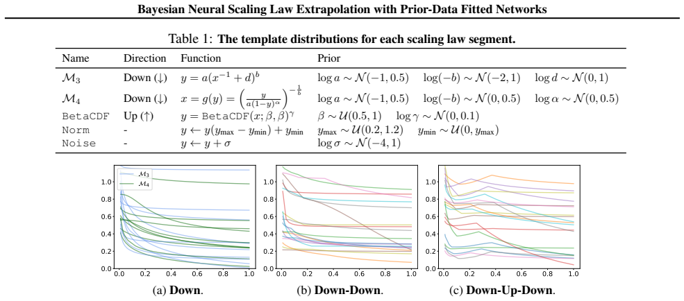
The load-bearing object is the neural scaling law prior: a hierarchical generative process in which each curve is stitched from segments. Downward segments are drawn from M3, $y=a(x-1+d)^b$, or M4, whose inverse form is $x = (y/(a(1-y)^{\alpha}))^{-1/b}$ with $c=0$ and $y_0=1$; upward segments use a Beta CDF with an S-shape; the number and locations of breaks are sampled randomly; each segment is renormalized and noise is added. A cutoff distribution then fixes which part of the curve is context and which is target, deliberately excluding cutoffs after which a surprise break is judged unpredictable. Training the PFN on 1.6 million such synthetic curves with an autoregressive context loss plus an interpolation variant gives the network the inductive bias to extrapolate power-law tails, infer breaks automatically, and quantify uncertainty without closed-form posteriors.
What would settle it
Generate a family of scaling curves that is structurally absent from the Section 3.1 prior—for example, an exponential saturation curve with a long flat plateau at both ends, or a curve that keeps rising after a downward segment—and compare NSL-PFN against MCMC(BNSL) on RMSLE and MSCE; if NSL-PFN loses calibration or accuracy on these out-of-prior shapes, the prior-support assumption marks the limits of the claim.
Extended reading notes
Core claim
The central claim, stated on the paper's own terms, is that a meta-learned in-context Bayesian model with a scaling-law-shaped prior outperforms both classical parametric point estimates and the natural MCMC baselines at predicting the unseen tail of neural scaling curves. The method, NSL-PFN, ingests the observed portion of a curve as context and returns a full predictive distribution at extrapolated inputs, so it simultaneously supplies a point fit (the median), a functional form, an inferred number of breaks, and calibrated uncertainty. Empirically the paper reports the best average RMSLE and log-likelihood among all compared methods on the image classification benchmark, the NLP/Nano suite, and the ColPret and double-descent datasets, and the best MSCE calibration on ColPret and DD. The authors further claim that these uncertainties drive effective Bayesian active learning, selecting the next observation point by variation ratio, and that the whole inference costs a single forward pass per curve.
Load-bearing premise
The evaluation curves are all within the support of the manually designed prior, which was tuned by eye to match those same benchmarks, so the method's edge may depend on the prior already knowing the curve shapes.
Editorial extensions
If this is right
- A single forward pass per curve replaces per-curve fitting, cutting inference from tens to hundreds of seconds (M4/BNSL/MCMC) to about 0.02 seconds while improving fit accuracy.
- Small-scale observed context suffices to forecast the tail with a predictive distribution, so compute-budget decisions can weigh expected gain against cost and risk.
- The model infers the number of breaks and the functional form implicitly, removing the cross-validation step that BNSL requires.
- In Bayesian active learning, uncertainty-based selection of the next observation point improves predictive likelihood over MCMC baselines as more points are collected.
- On double-descent curves, the method predicts the eventual downturn even when the context ends in an upward segment, which MCMC(BNSL) does not do.
Reading between the lines
- The same trained network might transfer to other break-prone extrapolation problems, such as learning curves in AutoML or hardware and financial scaling, where the segment structure applies.
- Since the prior hyperparameters were manually fitted to the benchmark shapes, meta-learning or adapting them from the observed context would be a natural extension that could make the method robust to new curve families.
- The cutoff restriction encodes a strong inductive assumption: after a downward segment, a future break is treated as unpredictable, and measuring whether predictive uncertainty rises on curves with late breaks would quantify what that assumption costs.
- The interpolation objective opens a route to using the model as a multi-fidelity surrogate, deciding experimentally which scale to measure next rather than only extrapolating tails.
Editorial analysis
A structured set of objections, weighed in public.
Referee Report
Summary. The paper proposes NSL-PFN, a Prior-data Fitted Network for Bayesian neural scaling law extrapolation. The authors design a functional prior over scaling-law curves by concatenating M3/M4 power-law segments with random breaks and occasional upward BetaCDF segments, then train a Transformer to output posterior predictive distributions. The method is evaluated on image classification (IC), NLP, nanoGPT-Bench (Nano), ColPret, and double-descent (DD) datasets against M1--M4 and BNSL point estimators, MCMC variants of these models, LC-PFN, BLR, and DKGP. The central claims are that NSL-PFN gives better point predictions (RMSLE) and better uncertainty quantification (log-likelihood and MSCE) than the baselines, especially in data-limited settings, and that its amortized inference is far cheaper than MCMC.
Significance. If the central claims hold, this is a practically useful contribution: it provides fast, uncertainty-aware extrapolation for neural scaling laws, with code and models released. The empirical effort is substantial: six benchmark suites, calibration metrics, active-learning experiments, ablations of the prior components, and an analysis of MCMC sample counts. The main reservation is that the functional prior was tuned on the evaluation data themselves, so the reported gains may largely reflect prior coverage of the test class rather than general extrapolation ability. Because the PFN is entirely defined by its prior, this is a load-bearing concern for the paper's main claim.
major comments (4)
- [§4.3, Table 1, Fig. 7] The evaluation protocol is circular for the paper's central claim. Section 4.3 states that the prior hyperparameters in Table 1 were 'manually adjusted to visually match the shapes of the actual curves collected from various domains' and then further optimized by Bayesian optimization on the average RMSLE of the same benchmarks (Fig. 7, Table 13). Since the PFN is trained exclusively on samples from this prior, using the evaluation curves to set the prior means the results in Tables 2-4, Fig. 3, and Table 9 partly measure how well the prior was fit to the test class. Please add a genuinely out-of-prior evaluation: fix the prior without inspecting the evaluation curves, or hold out entire scaling-law families or datasets during prior tuning, and report RMSLE, LL, and MSCE on those held-out curves. Without this, the abstract's 'superior performance' claim is not supportable beyond the tuned benchmark suite.
- [§3.1 (cutoff distribution) and §4.1/Fig. 4] The cutoff restrictions exclude from training exactly the data-limited scenarios that are later evaluated. Down-Down curves only allow cutoffs within the last segment, and Down-Up-Down curves only allow cutoffs in the second or third segment; however, the DD evaluations in Fig. 4 and Figs. 16-23 include 40% cutoffs in which the context lies entirely in the first decreasing segment before the upward break. For such inputs the model has never seen a valid training context of that shape, so the reported DD results at low cutoffs are out-of-support predictions. Please either train with cutoffs before the first break, or explicitly restrict and clearly label the DD evaluation to contexts that are within the training cutoff support. The 'inherently difficult' argument in §4.1 does not resolve the mismatch between the training distribution and the evaluation distribution.
- [§C, Eq. (11) and Table 10] The BNSL baseline is not evaluated with the method as described by Eq. (5). The implementation in Eq. (11) is a neural-network reparameterization, and the number of breaks and validation procedure are a reimplementation based on the paper description, with four variants compared in Table 10. This means the BNSL and MCMC(BNSL) results in Tables 2-4 may not reflect the actual BNSL method. Please use the official implementation if one is available; otherwise, report which variant was used and justify why it is the fairest, and provide failure counts for the excluded trials.
- [§C, Table 11] The MCMC baselines use priors that appear poorly calibrated and possibly invalid, e.g., loga ~ U(1,1000) for MCMC(M4) and a ~ U(-1,0.5) for MCMC(M1) despite positive-valued targets. Such priors can produce extremely diffuse or invalid proposals and may handicap the Bayesian baselines. This is important because the paper's claim of superiority over Bayesian baselines rests on these comparisons. Please report results with more standard, clearly justified priors, or include a sensitivity analysis over prior choices.
minor comments (4)
- [Table 4] The footnote '† indicates that some trials failed due to overflow error, which were excluded from the calculation' should specify how many trials failed, for which methods and datasets, and whether the reported averages and standard deviations are over the remaining trials only.
- [§3.2 and §4.2] The interpolation-loss training procedure is described only briefly ('randomly sample a subset of T to add them to C'). Please specify the distribution over the number or fraction of target points moved to the context, as this affects the active-learning model and reproducibility.
- [Fig. 6] The caption states that convergence failures were observed for some MCMC(BNSL) runs and that these runs were excluded; please report the number of excluded runs at each sample count, since selective exclusion can bias the comparison.
- [§C, Table 11] The MCMC priors are not matched across baselines: for example, MCMC(M4) uses a different x-normalization (maximum 1000) from the other MCMC variants. Please justify this asymmetry or use a common normalization.
Circularity Check
Prior hyperparameters were tuned to the evaluation curves, so the reported extrapolation gains partly measure in-prior fit rather than independent predictive skill.
-
self definitional
[Section 4.3 (Prior hyperparameter tuning) and Appendix D (Hyperparameter Tuning for Prior Distributions), with Tables 1 and 13 and Figure 7.]
"For our prior design, we manually adjust the parameters of our functional prior to visually match the shapes of the actual curves collected from various domains. ... We conduct a simple Bayesian optimization (BO) on the prior parameters to minimize the average RMSLE over 60 BO steps."
The PFN posterior predictive is trained entirely on synthetic curves sampled from this functional prior (Section 3.1, Eq. 8-10). The prior's hyperparameters were then manually matched to and numerically optimized against the same benchmark curves used for evaluation, with the optimization objective being the average RMSLE, the paper's main evaluation metric. Consequently, the reported RMSLE, log-likelihood, and calibration results on IC, NLP, Nano, ColPret, and DD measure how well the hand-tuned prior covers those specific curves, not independent extrapolation to unseen scaling-law families. The 'prediction' is partly a reconstruction from a distribution whose parameters were selected using the target values of those same curves, and no out-of-prior evaluation is provided.
full rationale
The central empirical claim is partially circular because the functional prior is not fixed a priori: Section 4.3 states the prior parameters were manually adjusted to visually match the actual evaluation curves, and Appendix D confirms that Bayesian optimization minimized the average RMSLE over 60 steps on those same benchmarks. Since the PFN is meta-trained solely on samples from this prior, its test-time predictions on those datasets are in-distribution for a prior fit to the test targets; the reported superiority therefore conflates genuine amortized Bayesian inference with prior coverage engineered from the evaluation data. This is a specific, quotable reduction of the evaluation metric into the prior-selection objective, warranting a score of 6 rather than a minor-citation score. No load-bearing self-citation or imported uniqueness theorem is present: comparisons to LC-PFN and MCMC baselines are external and independently implemented. A separate, non-circular limitation is the cutoff restriction in Section 3.1, which excludes contexts ending before a future break, yet the DD evaluation at early cutoffs includes such cases; this makes some evaluations harder for NSL-PFN rather than easier, and is noted as a validity concern, not as additional circularity.
Assumptions & free parameters
free parameters (4)
- M3 prior hyperparameters (log a, log(-b), log d means and stds) =
as in Table 1: N(-1,0.5), N(-2,1), N(0,1)
- M4 prior hyperparameters (log a, log(-b), log alpha means and stds) =
as in Table 1: N(-1,0.5), N(0,0.5), N(0,0.5)
- BetaCDF, Norm, and Noise hyperparameters =
beta ~ U(0.5,1), log gamma ~ N(0,0.1), ymax ~ U(0.2,1.2), ymin ~ U(0,ymax), log sigma ~ N(-4,1)
- Function family mixture probabilities and break probabilities =
not specified in the paper
assumptions (5)
- domain assumption Neural scaling laws are generated by piecewise segments drawn from M3, M4, and BetaCDF
- domain assumption Cutoff restriction: no unexpected breaks after a downward last segment; an upward last segment eventually turns downward
- standard math PFN training objective (Eq. 8-10) minimizes expected KL to the true posterior predictive
- domain assumption Amortized inference transfers from synthetic prior data to real scaling curves
- ad hoc to paper Rejection sampling of curves: negative y or NaN values are discarded
Cite this review
Pith. "Pith review of Bayesian Neural Scaling Law Extrapolation with Prior-Data Fitted Networks." pith.science (2026). https://pith.science/paper/EXP43WHQ
@misc{pith2026250523032,
  author       = {Pith},
  title        = {Pith review of: Bayesian Neural Scaling Law Extrapolation with Prior-Data Fitted Networks},
  year         = {2026},
  howpublished = {\url{https://pith.science/paper/EXP43WHQ}},
  note         = {Machine review of arXiv:2505.23032}
}
read the original abstract
Scaling has been a major driver of recent advancements in deep learning. Numerous empirical studies have found that scaling laws often follow the power-law and proposed several variants of power-law functions to predict the scaling behavior at larger scales. However, existing methods mostly rely on point estimation and do not quantify uncertainty, which is crucial for real-world applications involving decision-making problems such as determining the expected performance improvements achievable by investing additional computational resources. In this work, we explore a Bayesian framework based on Prior-data Fitted Networks (PFNs) for neural scaling law extrapolation. Specifically, we design a prior distribution that enables the sampling of infinitely many synthetic functions resembling real-world neural scaling laws, allowing our PFN to meta-learn the extrapolation. We validate the effectiveness of our approach on real-world neural scaling laws, comparing it against both the existing point estimation methods and Bayesian approaches. Our method demonstrates superior performance, particularly in data-limited scenarios such as Bayesian active learning, underscoring its potential for reliable, uncertainty-aware extrapolation in practical applications.
Figures


Figures from the paper (20 more)


Reference graph
Works this paper leans on
-
[1]
Exploring the limits of large scale pre-training.arXiv preprint arXiv:2110.02095,
Abnar, S., Dehghani, M., Neyshabur, B., and Sedghi, H. Exploring the limits of large scale pre-training.arXiv preprint arXiv:2110.02095,
-
[3]
Since the range of x for the prior was sampled from [0, 100] during LC-PFN training, we normalize x-values to the same range during inference. LC-PFN includes its own normalization method for y-values, enabling it to predict learning curves across various ranges and directions. However, when evaluating LC-PFN on scaling laws, we found that its normalizati...
work page 2021
-
[4]
20 40 60 80 100 120 .4 .5 .6T est Error 20 40 60 80 100 120 .4 .5 .6 20 40 60 80 100 120 .4 .5 .6 20 40 60 80 100 120 .4 .5 .6 Context T arget Cutoff MCMC (BNSL) 20 40 60 80 100 120 .4 .5 .6T est Error 20 40 60 80 100 120 .4 .5 .6 20 40 60 80 100 120 .4 .5 .6 20 40 60 80 100 120 .4 .5 .6 Context T arget Cutoff LC-PFN 20 40 60 80 100 120 Model Width .4 .5 ...
work page 2021
-
[10]
Devlin, J. Bert: Pre-training of deep bidirectional trans- formers for language understanding.arXiv preprint arXiv:1810.04805,
-
[12]
The llama 3 herd of models.arXiv preprint arXiv:2407.21783,
Dubey, A., Jauhri, A., Pandey, A., Kadian, A., Al-Dahle, A., Letman, A., Mathur, A., Schelten, A., Yang, A., Fan, A., et al. The llama 3 herd of models.arXiv preprint arXiv:2407.21783,
-
[14]
Gargiani, M., Klein, A., Falkner, S., and Hutter, F. Proba- bilistic rollouts for learning curve extrapolation across hy- perparameter settings.arXiv preprint arXiv:1910.04522,
arXiv 1910
-
[15]
Scaling laws for neural machine translation.arXiv preprint arXiv:2109.07740,
Ghorbani, B., Firat, O., Freitag, M., Bapna, A., Krikun, M., Garcia, X., Chelba, C., and Cherry, C. Scaling laws for neural machine translation.arXiv preprint arXiv:2109.07740,
-
[16]
Gordon, M. A., Duh, K., and Kaplan, J. Data and parameter scaling laws for neural machine translation. InProceed- ings of the 2021 Conference on Empirical Methods in Natural Language Processing, pp. 5915–5922,
work page 2021
Show all 58 references
-
[17]
and Dao, T
Gu, A. and Dao, T. Mamba: Linear-time sequence modeling with selective state spaces.arXiv preprint arXiv:2312.00752,
-
[19]
Hoffmann, J., Borgeaud, S., Mensch, A., Buchatskaya, E., Cai, T., Rutherford, E., Casas, D. d. L., Hendricks, L. A., Welbl, J., Clark, A., et al. Training compute-optimal large language models.arXiv preprint arXiv:2203.15556,
-
[20]
Tabpfn: A transformer that solves small tabu- lar classification problems in a second.arXiv preprint arXiv:2207.01848,
Hollmann, N., M ¨uller, S., Eggensperger, K., and Hut- ter, F. Tabpfn: A transformer that solves small tabu- lar classification problems in a second.arXiv preprint arXiv:2207.01848,
-
[21]
Bayesian active learning for classification and preference learning.arXiv preprint arXiv:1112.5745,
Houlsby, N., Husz´ar, F., Ghahramani, Z., and Lengyel, M. Bayesian active learning for classification and preference learning.arXiv preprint arXiv:1112.5745,
-
[23]
B., Chess, B., Child, R., Gray, S., Radford, A., Wu, J., and Amodei, D
Kaplan, J., McCandlish, S., Henighan, T., Brown, T. B., Chess, B., Child, R., Gray, S., Radford, A., Wu, J., and Amodei, D. Scaling laws for neural language models. arXiv preprint arXiv:2001.08361,
2001 arXiv
-
[24]
Kingma, D. P. Adam: A method for stochastic optimization. arXiv preprint arXiv:1412.6980,
-
[25]
Big transfer (bit): General vi- sual representation learning
Kolesnikov, A., Beyer, L., Zhai, X., Puigcerver, J., Yung, J., Gelly, S., and Houlsby, N. Big transfer (bit): General vi- sual representation learning. InComputer Vision–ECCV 2020: 16th European Conference, Glasgow, UK, Au- gust 23–28, 2020, Proceedings, Part V 16, pp. 491–507...
2020
-
[27]
and van Rijn, J
Mohr, F. and van Rijn, J. N. Learning curves for decision making in supervised machine learning–a survey.arXiv preprint arXiv:2201.12150,
-
[29]
Deep double descent: Where bigger models and more data hurt.Journal of Statistical Mechan- ics: Theory and Experiment, 2021(12):124003,
Nakkiran, P., Kaplun, G., Bansal, Y ., Yang, T., Barak, B., and Sutskever, I. Deep double descent: Where bigger models and more data hurt.Journal of Statistical Mechan- ics: Theory and Experiment, 2021(12):124003,
2021
-
[30]
In-context freeze-thaw bayesian optimization for hyperparameter optimization
Rakotoarison, H., Adriaensen, S., Mallik, N., Garibov, S., Bergman, E., and Hutter, F. In-context freeze-thaw bayesian optimization for hyperparameter optimization. arXiv preprint arXiv:2404.16795,
-
[31]
Rosenfeld, J. S. Scaling laws for deep learning.arXiv preprint arXiv:2108.07686,
-
[32]
S., Rosenfeld, A., Belinkov, Y ., and Shavit, N
Rosenfeld, J. S., Rosenfeld, A., Belinkov, Y ., and Shavit, N. A constructive prediction of the generalization error across scales.arXiv preprint arXiv:1909.12673,
1909 arXiv
-
[33]
Sharma, U
doi: 10.1007/s11263-015-0816-y. Sharma, U. and Kaplan, J. Scaling laws from the data mani- fold dimension.Journal of Machine Learning Research, 23(9):1–34,
-
[34]
Swersky, K., Snoek, J., and Adams, R. P. Freeze-thaw bayesian optimization.arXiv preprint arXiv:1406.3896,
-
[35]
Efficientnet: Rethinking model scaling for convolu- tional neural networks.arXiv preprint arXiv:1905.11946,
Tan, M. Efficientnet: Rethinking model scaling for convolu- tional neural networks.arXiv preprint arXiv:1905.11946,
1905 arXiv
-
[36]
Lamda: Language models for dialog appli- cations.arXiv preprint arXiv:2201.08239,
Thoppilan, R., De Freitas, D., Hall, J., Shazeer, N., Kul- shreshtha, A., Cheng, H.-T., Jin, A., Bos, T., Baker, L., Du, Y ., et al. Lamda: Language models for dialog appli- cations.arXiv preprint arXiv:2201.08239,
-
[37]
Llama: Open and efficient foundation lan- guage models.arXiv preprint arXiv:2302.13971, 2023a
12 Bayesian Neural Scaling Law Extrapolation with Prior-Data Fitted Networks Touvron, H., Lavril, T., Izacard, G., Martinet, X., Lachaux, M.-A., Lacroix, T., Rozi`ere, B., Goyal, N., Hambro, E., Azhar, F., et al. Llama: Open and efficient foundation lan- guage models.arXiv pre...
-
[38]
Verdenius, S., Zerio, A., and Wang, R. L. Lat-pfn: A joint embedding predictive architecture for in-context time-series forecasting.arXiv preprint arXiv:2405.10093,
-
[39]
13 Bayesian Neural Scaling Law Extrapolation with Prior-Data Fitted Networks A. More Discussion on Related Work Neural scaling lawsThere are many observations that neural scaling laws are empirically predictable (Hestness et al., 2017; Johnson et al., 2018; Rosenfeld et al., 2...
2017
-
[40]
Alabdulmohsin et al
to guarantee that the power law function converges to a finite constant when the domain of interest approaches to infinity. Alabdulmohsin et al. (2022) have proposed M4 to handle non-power law behaviour in partial scaling law. More recently, Caballero et al. (2022) have propos...
2022
-
[41]
point estimates
primarily modeled learning curves (LCs) based on dataset size, providing “point estimates” of performance without a probabilistic nature, let alone a Bayesian framework for uncertainty quantification. Additionally, these models often do not address deep neural network (DNN) tr...
2015
-
[42]
For each downstream task, the benchmark provides 18 scaling law variations (2 model sizes × 3 model types × 3 few-shot settings), resulting in a total of 72 scaling laws
dataset and tested on downstream tasks:ImageNet(Russakovsky et al., 14 Bayesian Neural Scaling Law Extrapolation with Prior-Data Fitted Networks 2015),CIFAR-100(Krizhevsky et al., 2009),Birds(Welinder et al., 2010), andCaltech101(Fei-Fei et al., 2004). For each downstream task...
2015
-
[43]
is evaluated on next-token prediction. Scaling laws are provided for five different parameter sizes, with the x-axis indicating the number of observed examples and the y-axis showing the validation loss, rescaled to the range [0, 1]. For the BB task, the one-shot and two-shot ...
2023
-
[44]
nanoGPT-Bench (Nano) is a benchmark introduced in (Kadra et al., 2023), which evaluates the performance of nanoGPT trained on the OpenWebText dataset (Gokaslan et al.,
to enhance the analysis of scaling behavior in the NLP domain, focusing on factors beyond the number of observed examples. nanoGPT-Bench (Nano) is a benchmark introduced in (Kadra et al., 2023), which evaluates the performance of nanoGPT trained on the OpenWebText dataset (Gok...
2023
-
[45]
Both the final and best performance are reported, resulting in a total of 24 scaling laws
using 12 different hyperparameter configurations. Both the final and best performance are reported, resulting in a total of 24 scaling laws. In this benchmark, the x-axis corresponds to the model embedding size, while the y-axis represents either the final or best validation l...
2021
-
[46]
In these scaling laws, the x-axis represents either the model embedding size or the number of observed examples, while the y-axis reflects the test error or cross-entropy test loss
that illustrate double descent behavior (DD). In these scaling laws, the x-axis represents either the model embedding size or the number of observed examples, while the y-axis reflects the test error or cross-entropy test loss. C. Implementation Details M1−4.For experiments in...
2022
-
[47]
authors. The implementation of the code has minor adjustments to ensure stable and efficient training, as detailed below: BNSL:y= exp log efbnsl(˜x)+e a +y mean ! , wheref bnsl(˜x) =W3 · W2 ·softplus(W 1 ˜x+b1) +b 2 +b 3, ˜x= log(x)−µ x σx , µx =mean(log(x train)), σ x =std(lo...
2013
-
[48]
Hyperparameters, including those of the neural network used as the basis function for BLR, are tuned via marginal log-likelihood
with neural network basis functions, BLR with polynomial basis functions, BLR with RBF basis functions, BLR with Fourier basis functions, BLR with sigmoid basis functions, BLR with spline basis functions, and DKGP (Wilson et al., 2016). Hyperparameters, including those of the ...
2016
-
[49]
As shown in Table 12, BLR models with predefined basis functions exhibit significant performance degradation
with a learning rate of 0.01. As shown in Table 12, BLR models with predefined basis functions exhibit significant performance degradation. LC-PFNFor our experiments, we utilize the LC-PFN as described in Adriaensen et al. (2023)
2023
-
[52]
20 40 60 80 100 120 .5 .6 .7T est Error 20 40 60 80 100 120 .5 .6 .7 20 40 60 80 100 120 .5 .6 .7 20 40 60 80 100 120 .5 .6 .7 Context T arget Cutoff MCMC (BNSL) 20 40 60 80 100 120 .5 .6 .7T est Error 20 40 60 80 100 120 .5 .6 .7 20 40 60 80 100 120 .5 .6 .7 20 40 60 80 100 1...
2021
-
[53]
20 40 60 80 100 120 .5 .6 .7T est Error 20 40 60 80 100 120 .5 .6 .7 20 40 60 80 100 120 .5 .6 .7 20 40 60 80 100 120 .5 .6 .7 Context T arget Cutoff MCMC (BNSL) 20 40 60 80 100 120 .5 .6 .7T est Error 20 40 60 80 100 120 .5 .6 .7 20 40 60 80 100 120 .5 .6 .7 20 40 60 80 100 1...
2021
-
[54]
10 20 30 40 50 60 .3 .4 .5T est Error 10 20 30 40 50 60 .3 .4 .5 10 20 30 40 50 60 .3 .4 .5 10 20 30 40 50 60 .3 .4 .5 Context T arget Cutoff MCMC (BNSL) 10 20 30 40 50 60 .3 .4 .5T est Error 10 20 30 40 50 60 .3 .4 .5 10 20 30 40 50 60 .3 .4 .5 10 20 30 40 50 60 .3 .4 .5 Cont...
2021
-
[55]
25000 50000 75000 100000125000 5 7 10 12T est Loss 25000 50000 75000 100000125000 5 7 10 12 25000 50000 75000 100000125000 5 7 10 12 25000 50000 75000 100000125000 5 7 10 12 Context T arget Cutoff MCMC (BNSL) 25000 50000 75000 100000125000 5 7 10 12T est Loss 25000 50000 75000...
2021
-
[56]
50 100 150 200 8 10 12 14T est Loss 50 100 150 200 8 10 12 14 50 100 150 200 8 10 12 14 50 100 150 200 8 10 12 14 Context T arget Cutoff MCMC (BNSL) 50 100 150 200 8 10 12 14T est Loss 50 100 150 200 8 10 12 14 50 100 150 200 8 10 12 14 50 100 150 200 8 10 12 14 Context T arge...
2021
-
[57]
100 200 300 400 500 4 5 6 7T est Loss 100 200 300 400 500 4 5 6 7 100 200 300 400 500 4 5 6 7 100 200 300 400 500 4 5 6 7 Context T arget Cutoff MCMC (BNSL) 100 200 300 400 500 4 5 6 7T est Loss 100 200 300 400 500 4 5 6 7 100 200 300 400 500 4 5 6 7 100 200 300 400 500 4 5 6 ...
2021
-
[58]
10 20 30 40 50 60 .5 .6 .7 .8 .9T est Error 10 20 30 40 50 60 .5 .6 .7 .8 .9 10 20 30 40 50 60 .5 .6 .7 .8 .9 10 20 30 40 50 60 .5 .6 .7 .8 .9 Context T arget Cutoff MCMC (BNSL) 10 20 30 40 50 60 .5 .6 .7 .8 .9T est Error 10 20 30 40 50 60 .5 .6 .7 .8 .9 10 20 30 40 50 60 .5 ....
2021
-
[2003]
P., Grabocka, J., and Hutter, F
M¨uller, S., Hollmann, N., Arango, S. P., Grabocka, J., and Hutter, F. Transformers can do bayesian inference.arXiv preprint arXiv:2112.10510,
-
[2006]
Bojar, O., Buck, C., Federmann, C., Haddow, B., Koehn, P., Leveling, J., Monz, C., Pecina, P., Post, M., Saint- Amand, H., et al
ISBN 0387310738. Bojar, O., Buck, C., Federmann, C., Haddow, B., Koehn, P., Leveling, J., Monz, C., Pecina, P., Post, M., Saint- Amand, H., et al. Findings of the 2014 workshop on statistical machine translation. InProceedings of the ninth workshop on statistical machine trans...
2014
-
[2011]
Pre- dicting accuracy on large datasets from smaller pilot data
Johnson, M., Anderson, P., Dras, M., and Steedman, M. Pre- dicting accuracy on large datasets from smaller pilot data. In56th Annual Meeting of the Association for Computa- tional Linguistics, ACL 2018, pp. 450–455. Association for Computational Linguistics (ACL),
2018
-
[2012]
and Lane, I
Chandrashekaran, A. and Lane, I. R. Speeding up hyper- parameter optimization by extrapolation of learning curves using previous builds. InMachine Learning and Knowledge Discovery in Databases: European Confer- ence, ECML PKDD 2017, Skopje, Macedonia, Septem- ber 18–22, 2017, ...
2017
-
[2014]
Brown, T. B. Language models are few-shot learners.arXiv preprint arXiv:2005.14165,
2005 arXiv
-
[2015]
A survey on in-context learning
Dong, Q., Li, L., Dai, D., Zheng, C., Wu, Z., Chang, B., Sun, X., Xu, J., and Sui, Z. A survey on in-context learning. arXiv preprint arXiv:2301.00234,
-
[2017]
How much data is needed to train a medical image deep learning sys- tem to achieve necessary high accuracy?arXiv preprint arXiv:1511.06348,
Cho, J., Lee, K., Shin, E., Choy, G., and Do, S. How much data is needed to train a medical image deep learning sys- tem to achieve necessary high accuracy?arXiv preprint arXiv:1511.06348,
-
[2018]
B., Zhang, A
Lee, D. B., Zhang, A. S., Kim, B., Park, J., Lee, J., Hwang, S. J., and Lee, H. B. Cost-sensitive multi-fidelity bayesian optimization with transfer of learning curve extrapolation. arXiv preprint arXiv:2405.17918,
-
[2019]
Learning generative visual models from few training examples: An incremen- tal bayesian approach tested on 101 object categories
Fei-Fei, L., Fergus, R., and Perona, P. Learning generative visual models from few training examples: An incremen- tal bayesian approach tested on 101 object categories. In 2004 conference on computer vision and pattern recogni- tion workshop, pp. 178–178. IEEE,
2004
-
[2020]
Broken neural scaling laws.arXiv preprint arXiv:2210.14891,
Caballero, E., Gupta, K., Rish, I., and Krueger, D. Broken neural scaling laws.arXiv preprint arXiv:2210.14891,
-
[2021]
L., Almeida, D., Altenschmidt, J., Altman, S., Anadkat, S., et al
Achiam, J., Adler, S., Agarwal, S., Ahmad, L., Akkaya, I., Aleman, F. L., Almeida, D., Altenschmidt, J., Altman, S., Anadkat, S., et al. Gpt-4 technical report.arXiv preprint arXiv:2303.08774,
-
[2022]
An image is worth 16x16 words: Transformers for image recognition at scale.arXiv preprint arXiv: 2010.11929,
Alexey, D. An image is worth 16x16 words: Transformers for image recognition at scale.arXiv preprint arXiv: 2010.11929,
2010 arXiv
-
[2023]
Hestness, J., Narang, S., Ardalani, N., Diamos, G., Jun, H., Kianinejad, H., Patwary, M. M. A., Yang, Y ., and Zhou, Y . Deep learning scaling is predictable, empirically.arXiv preprint arXiv:1712.00409,
-
[2024]
10 Bayesian Neural Scaling Law Extrapolation with Prior-Data Fitted Networks Chung, H
URL https: //arxiv.org/abs/2410.11840. 10 Bayesian Neural Scaling Law Extrapolation with Prior-Data Fitted Networks Chung, H. W., Hou, L., Longpre, S., Zoph, B., Tay, Y ., Fe- dus, W., Li, Y ., Wang, X., Dehghani, M., Brahma, S., et al. Scaling instruction-finetuned language m...
Reviewed August 7, 2026 · model on record in the stance chip above.
Discussion (0). Sign in to comment.