REVIEW 2 major objections 4 minor 33 references
Leveraging machine learning features for linear optical interferometer control
T0 review · 2 major / 4 minor · reviewed 2026-08-07 · deepseek-v4-flash
Pith's one-line read Machine learning turns interferometer control into linear algebra.
desk verdict Promising linearization idea for interferometer control, but the shared-pseudoinverse claim is wrong and the sample-complexity figures don't match the equations. read the letter →
The pith
A machine-rendered reading of the paper's core claim, the machinery that carries it, and where it could break.
The reading
What carries the argument
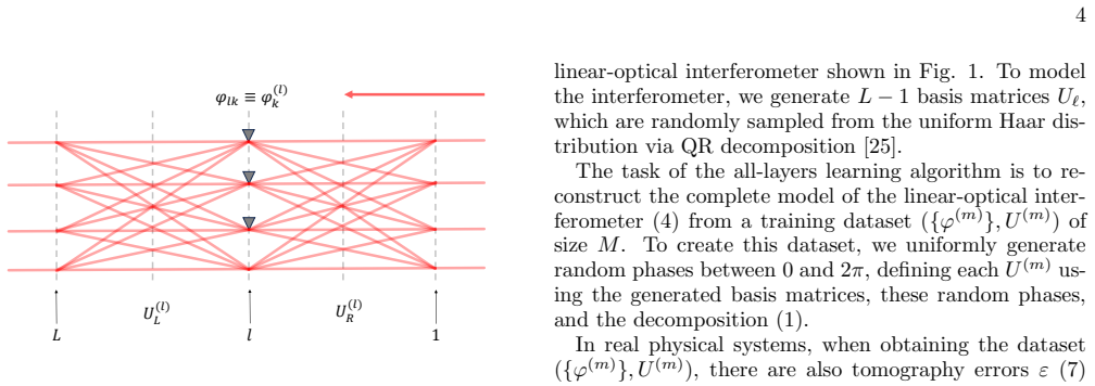
The key object is the monomial feature expansion of Eq. (4), $u_{ij} = \sum_{\bar{k}} w_{i\bar{k}j}\,\theta_{i\bar{k}j}$, with $\theta$ formed by products of the phase exponentials. It converts device identification into a linear least-squares fit with feature matrix $\Theta$, whose pseudoinverse is computed once. For layer-wise training, the features shrink to the single-layer phase exponentials, giving $O(N)$ tomography samples per layer.
What would settle it
Apply the training procedure to a device with deliberately coupled phase shifters, where setting $\varphi_k$ also shifts a neighboring phase. If the model error on held-out phases cannot be reduced below a floor no matter how large the training sample is, the monomial-feature linearization is violated.
Extended reading notes
Core claim
The central discovery is that for an interferometer written as a product $U = \Phi_L U_{L-1} \cdots U_1 \Phi_1$, every matrix element $u_{ij}$ is exactly a scalar product of a weight vector $w_{i\bar{k}j}$ and a feature vector $\theta_{i\bar{k}j}$ whose entries are products of phase exponentials $e^{i\varphi}$ along paths from input $i$ to output $j$. The weights are products of the fixed basis-matrix elements and fully characterize the device; the features depend only on the phase settings. Given $M$ tomographed unitaries at random phase settings, the weights follow from one Moore-Penrose pseudoinverse, and phase programming of the model is then a small optimization. The paper also shows a layer-wise variant that applies to deeper circuits.
Load-bearing premise
The load-bearing premise is that the physical device is exactly a sequence of fixed mode-mixing layers and independent, phase-only shifters, so every phase enters only as $e^{i\varphi}$ and the tomographed unitaries are faithful.
Editorial extensions
If this is right
- Any interferometer of the layered form can be programmed from data without an analytic decomposition, so new or imperfect architectures become usable.
- For shallow circuits, a single tomography campaign suffices: after training, all future target unitaries are programmed by optimizing the model.
- For deep circuits, layer-by-layer alternating least squares works with $O(N)$ tomography samples per layer.
- Training error on the model falls as $1/M$ beyond a minimum sample size, so noise in tomography is diluted by more measurements.
- The programming phase no longer touches the physical device repeatedly, reducing wear and measurement overhead.
Reading between the lines
- A testable extension is to add coupling or crosstalk features to the model; if the monomial basis is expanded with interaction terms, the same linear framework could absorb small phase-shifter crosstalk.
- Because the model is linear, gradient-based programming could be replaced by closed-form updates for the single-layer case, potentially removing iterative optimization inside layer-wise training.
- Intensity-only characterization methods could be combined with the layer-wise scheme to avoid full phase-resolved tomography, at the cost of phase ambiguities.
Editorial analysis
A structured set of objections, weighed in public.
Referee Report
Summary. The paper proposes a supervised-learning framework for programming reconfigurable linear-optical interferometers. It observes that for an interferometer of the layered form U = Φ^L U^{L-1} ... U^1 Φ^1, each matrix element u_{ij} is a sum of monomials in the phase factors φ_k^{(ℓ)}, with coefficients (weights) composed of the fixed basis-matrix elements. This leads to two methods: an 'all-layers' method that trains the full weight tensor from a set of tomographed unitaries by solving a linear least-squares problem, and a 'layer-wise' method (alternating least squares) that trains a local linear model for each phase layer using O(N) samples per layer. Numerical simulations for Haar-random basis matrices show that the all-layers model fits after a minimum number M_min of training samples and that the test Frobenius error decreases as O(M^{-1}) and linearly with the tomography noise amplitude; the layer-wise method converges for full-depth interferometers with and without noise. The paper discusses limitations due to path-dependent loss and phase-shifter crosstalk.
Significance. If the proposed formulation were fully correct, the paper would offer a useful architecture-agnostic route to interferometer programming that avoids non-convex optimization for shallow circuits and uses cheap linear algebra. The algebraic expansion in Eq. (4) is exact and the numerical demonstrations are extensive, including noise scaling and the layer-wise ALS variant; the authors also state the main physical limitations explicitly. However, the central least-squares derivation contains a load-bearing inconsistency between the per-element feature definition and the claimed common pseudoinverse, and the sample-complexity threshold reported in the experiments does not follow from the equations as written. These issues need to be resolved before the central claim is established.
major comments (2)
- [Section III A, Eqs. (3)–(11)] The assertion that the matrix F in Eq. (11) is the same for all matrix elements (i,j) is not supported by the feature definition in Eq. (3). Since θ^{(m)}_{i\bar{k}j} contains the boundary phase factors φ^{(L,m)}_i and φ^{(1,m)}_j, the design matrix for fixed (i,j) is Θ_{ij} = D_{ij} Θ_0, where D_{ij}=diag_m(e^{i(φ^{(L,m)}_i+φ^{(1,m)}_j)}) and Θ_0 is common to all (i,j). The Moore–Penrose inverse is then F_{ij}= (Θ_0^*Θ_0)^{-1} Θ_0^* D_{ij}^*, which depends on (i,j) through D_{ij}; hence Eq. (11), which uses one F_{\bar{k}m} for every (i,j), is not the minimizer of the functional (10). If the authors instead solved a single multi-output least-squares problem with a global feature vector of length N^L, then Eq. (10) is not the objective being minimized, and the unconstrained solution does not enforce that each output (i,j) depends only on the N^{L-2} features θ_{i\bar{k}j}. The authors must state which formulation is intended and give the correct solution for that formulation.
- [Section IV A, Figs. 4–6] The reported minimum training sample size M_min=N^L (e.g., 1024 for N=4, L=5) is inconsistent with the per-element feature count from Eq. (3) and the functional (10), which contain N^{L-2} features per output and hence require only M ≥ N^{L-2} for generic phases. The numerical threshold suggests that the simulations actually solve a global least-squares problem with N^L features shared across outputs. The paper needs to reconcile this discrepancy, because the claimed sample-complexity scaling O(N^L) is a central quantity in the discussion of when all-layers learning is practical.
minor comments (4)
- [Eq. (9)] The Moore–Penrose solution for the overdetermined least-squares problem should be written as W=(Θ^*Θ)^{-1}Θ^*U (or W=Θ^†U); as displayed, (Θ^†Θ)^{-1}Θ^† equals Θ^† because Θ^†Θ is the identity, which is correct but obscures the intended normal equations. Please rewrite to avoid confusion.
- [Section III A, near Eq. (11)] The phrase 'the number of these features is O(N L)' should read O(N^L), or should explicitly distinguish the N^{L-2} features per output from the N^L features when counting over all (i,j).
- [Fig. 4 caption and Section IV A] M_min is used to mark the gray vertical line in Fig. 4 but is never formally defined; please state the criterion for 'successful learning' used to determine this threshold.
- [Eq. (15)] The notation 'x ∈ N(0,1)' should be 'x ∼ N(0,1)' for random variables; the same applies to y.
Circularity Check
No significant circularity: the learning pipeline is genuine supervised regression on an exact algebraic expansion, with self-citations only contextual.
full rationale
The derivation chain is self-contained. Equation (1) posits the device as alternating phase and mixing layers; Equation (3) is an exact algebraic expansion of each matrix element into monomial features theta and weights w (products of basis-matrix entries). Training then solves a least-squares regression (8)-(9) against tomographic measurements U^(m), which is a fitting step by design, not a hidden one: the resulting weights are not predictions of the training data but parameters of a model evaluated on held-out phase sets (Section IV A). The numerical test generates test unitaries from the same decomposition as the training data, which is standard in-distribution validation and does not make the claim circular. The architecture-agnostic motivation cites the authors' prior work [14,19], but these citations are contextual: [14] is a published universality/decomposition theorem that can be checked independently, and [19] is a prior algorithm being improved; neither defines the features, the loss, or the pseudoinverse solution. The paper explicitly concedes crosstalk and path-dependent loss as out-of-scope (Section V), which is a limitation, not a circular step. A separate correctness concern, namely that the claimed constancy of F across matrix elements in Eqs. (9)-(11) is false because the boundary phases make the design matrix depend on (i,j), calls for scrutiny, but even if Eq. (11) is misderived, that is an algebraic bug, not an equivalence between output and input. No step reduces a predicted quantity to a fitted input by construction.
Assumptions & free parameters
assumptions (4)
- domain assumption Any linear optical interferometer of the target class can be written as alternating phase-shift and mode-mixing layers, U = Phi_L U_{L-1} ... Phi_2 U_1 Phi_1, with phase-independent basis matrices U_l.
- domain assumption The phase shifters act independently, with no crosstalk and no path-dependent loss.
- domain assumption Full complex-valued unitary tomography is available for each training phase setting.
- standard math The feature columns are linearly independent for random phase settings, so the least-squares pseudoinverse in Eq. (9) is well-behaved.
Cite this review
Pith. "Pith review of Leveraging machine learning features for linear optical interferometer control." pith.science (2026). https://pith.science/paper/H3BHDTIE
@misc{pith2026250524032,
  author       = {Pith},
  title        = {Pith review of: Leveraging machine learning features for linear optical interferometer control},
  year         = {2026},
  howpublished = {\url{https://pith.science/paper/H3BHDTIE}},
  note         = {Machine review of arXiv:2505.24032}
}
read the original abstract
We have developed an algorithm that constructs a model of a reconfigurable optical interferometer, independent of specific architectural constraints. The programming of unitary transformations on the interferometer's optical modes relies on either an analytical method for deriving the unitary matrix from a set of phase shifts or an optimization routine when such decomposition is not available. Our algorithm employs a supervised learning approach, aligning the interferometer model with a training set derived from the device being studied. A straightforward optimization procedure leverages this trained model to determine the phase shifts of the interferometer with a specific architecture, obtaining the required unitary transformation. This approach enables the effective tuning of interferometers without requiring a precise analytical solution, paving the way for the exploration of new interferometric circuit architectures.
Figures


Figures from the paper (2 more)


Reference graph
Works this paper leans on
-
[19]
I. Kondratyev, V. Ivanova, S. Fldzhyan, A. Ar- genchiev, N. Kostyuchenko, S. Zhuravitskii, N. Skryabin, I. Dyakonov, M. Saygin, S. Straupe, A. Korneev, and S. Kulik, Large-scale error-tolerant programmable inter- ferometer fabricated by femtosecond laser writing, Pho- ton. Res. 12, A28 (2024)
work page 2024
- [21]
-
[1]
J. Carolan, C. Harrold, C. Sparrow, E. Martin-Lopez, N. J. Russell, J. W. Silverstone, P. J. Shadbolt, N. Mat- suda, M. Oguma, M. Itoh, G. D. Marshall, M. G. Thomp- son, J. C. F. Matthews, T. Hashimoto, J. L. O’Brien, and A. Laing, Universal linear optics, Science 349, 711 (2015)
work page 2015
-
[2]
(13) This numerical optimization problem can be solved us- ing methods such as gradient descent or the BFGS algo- rithm [24]. After performing this local minimization, we proceed to the next layer, conduct tomography, and train a local linear model (4). The advantage of this approach is that the sample size for training scales linearly as O(N ). However, ...
-
[3]
(16) To investigate the properties of the learning algorithm, we use averaged results based on the Frobenius met- ric across many samples of linear-optical interferometers, training datasets, and test evaluations. Fig. 4 shows the dependence of the Frobenius metric, averaged over 1000 samples of linear-optical interferom- eters, on the size M of the train...
-
[4]
N. C. Harris, J. Carolan, D. Bunandar, M. Prabhu, M. Hochberg, T. Baehr-Jones, M. L. Fanto, A. M. Smith, C. C. Tison, P. M. Alsing, and D. Englund, Linear programmable nanophotonic processors, Optica 5, 1623 (2018)
work page 2018
-
[5]
J. Wang, S. Paesani, Y. Ding, R. Santagati, P. Skrzypczyk, A. Salavrakos, J. Tura, R. Augusiak, L. Manˇ cinska, D. Bacco, D. Bonneau, J. W. Silverstone, Q. Gong, A. Ac ´ ın, K. Rottwitt, L. K. Oxenløwe, J. L. O’Brien, A. Laing, and M. G. Thompson, Multidimen- sional quantum entanglement with large-scale integrated optics, Science 360, 285 (2018)
work page 2018
-
[6]
J. Wang, F. Sciarrino, A. Laing, and M. G. Thompson, Integrated photonic quantum technologies, Nature Pho- tonics 14, 273 (2019)
work page 2019
Show all 33 references
-
[7]
Zhang, M
H. Zhang, M. Gu, X. D. Jiang, J. Thompson, H. Cai, S. Paesani, R. Santagati, A. Laing, Y. Zhang, M. H. Yung, Y. Z. Shi, F. K. Muhammad, G. Q. Lo, X. S. Luo, B. Dong, D. L. Kwong, L. C. Kwek, and A. Q. Liu, An op- tical neural chip for implementing complex-valued neural network...
2021 doi
-
[8]
Hamerly, L
R. Hamerly, L. Bernstein, A. Sludds, M. Soljaˇ ci´ c, and D. Englund, Large-scale optical neural networks based on photoelectric multiplication, Physical Review X 9, 10.1103/physrevx.9.021032 (2019)
2019 doi
-
[9]
Wetzstein, A
G. Wetzstein, A. Ozcan, S. Gigan, S. Fan, D. Englund, M. Soljaˇ ci´ c, C. Denz, D. A. B. Miller, and D. Psaltis, Inference in artificial intelligence with deep optics and photonics, Nature 588, 39 (2020)
2020
-
[10]
P´ erez-L´ opez, A
D. P´ erez-L´ opez, A. L´ opez, P. DasMahapatra, and J. Capmany, Multipurpose self-configuration of pro- grammable photonic circuits, Nature Communications 11, 10.1038/s41467-020-19608-w (2020)
2020 doi
-
[11]
A. Hurwitz, ¨ uber die erzeugung der invarianten durch integration, Nachrichten von der Gesellschaft der Wis- senschaften zu G¨ ottingen, Mathematisch-Physikalische Klasse 1897, 71 (1897)
-
[12]
M. Reck, A. Zeilinger, H. J. Bernstein, and P. Bertani, Experimental realization of any discrete unitary opera- tor, Phys. Rev. Lett. 73, 58 (1994)
1994
-
[13]
W. R. Clements, P. C. Humphreys, B. J. Metcalf, W. S. Kolthammer, and I. A. Walmsley, Optimal design for uni- versal multiport interferometers, Optica 3, 1460 (2016)
2016
-
[14]
Burgwal, W
R. Burgwal, W. R. Clements, D. H. Smith, J. C. Gates, W. S. Kolthammer, J. J. Renema, and I. A. Walmsley, Using an imperfect photonic network to implement ran- dom unitaries, Opt. Express 25, 28236 (2017)
2017
-
[15]
I. V. Dyakonov, I. A. Pogorelov, I. B. Bobrov, A. A. Kalinkin, S. S. Straupe, S. P. Kulik, P. V. Dyakonov, and S. A. Evlashin, Reconfigurable photonics on a glass chip, Phys. Rev. Applied 10, 044048 (2018)
2018
-
[16]
M. Y. Saygin, I. V. Kondratyev, I. V. Dyakonov, S. A. Mironov, S. S. Straupe, and S. P. Kulik, Robust archi- tecture for programmable universal unitaries, Phys. Rev. Lett. 124, 010501 (2020)
2020
-
[17]
S. A. Fldzhyan, M. Y. Saygin, and S. P. Kulik, Optimal design of error-tolerant reprogrammable multiport inter- ferometers, Optics Letters 45, 2632 (2020)
2020
-
[18]
S. A. Fldzhyan, M. Y. Saygin, and S. S. Straupe, Low- depth, compact, and error-tolerant photonic matrix- vector multiplication beyond the unitary group, Opt. Ex- press 32, 46239 (2024)
2024
-
[20]
Tillmann, C
M. Tillmann, C. Schmidt, and P. Walther, On unitary re- construction of linear optical networks, Journal of Optics 18, 114002 (2016)
2016
-
[22]
Bantysh, K
B. Bantysh, K. Katamadze, A. Chernyavskiy, and Y. Bogdanov, Fast reconstruction of programmable in- tegrated interferometers, Opt. Express 31, 16729 (2023)
2023
-
[23]
B. I. Bantysh, A. Y. Chernyavskiy, S. A. Fldzhyan, and Y. I. Bogdanov, Fast reconstruction of programmable interferometers with intensity-only measurements, Laser Physics Letters 21, 015203 (2023)
2023
-
[24]
Pearson, Liii
K. Pearson, Liii. on lines and planes of closest fit to sys- tems of points in space, The London, Edinburgh, and Dublin Philosophical Magazine and Journal of Science 2, 559 (1901). 8
1901
-
[25]
N. N. Skryabin, I. V. Dyakonov, M. Y. Saygin, and S. P. Kulik, Waveguide-lattice-based architecture for multi- channel optical transformations, Opt. Express 29, 26058 (2021)
2021
-
[26]
D. C. Liu and J. Nocedal, On the limited memory bfgs method for large scale optimization, Mathematical Pro- gramming 45, 503 (1989)
1989
-
[27]
Mezzadri, How to generate random matrices from the classical compact groups (2006), arXiv:math-ph/0609050 [math-ph]
F. Mezzadri, How to generate random matrices from the classical compact groups (2006), arXiv:math-ph/0609050 [math-ph]
2006 arXiv
-
[28]
Suess, N
D. Suess, N. Maraviglia, R. Kueng, A. Ma ¨ ınos, C. Spar- row, T. Hashimoto, N. Matsuda, D. Gross, and A. Laing, Rapid characterisation of linear-optical networks via PhaseLift, arXiv e-prints , arXiv:2010.00517 (2020), arXiv:2010.00517 [physics.optics]
2020 arXiv
-
[29]
Laing and J
A. Laing and J. L. O’Brien, Super-stable tomography of any linear optical device, arXiv e-prints , arXiv:1208.2868 (2012), arXiv:1208.2868 [quant-ph]
2012 arXiv
-
[30]
Rahimi-Keshari, M
S. Rahimi-Keshari, M. A. Broome, R. Fickler, A. Fedrizzi, T. C. Ralph, and A. G. White, Direct charac- terization of linear-optical networks, Optics Express 21, 13450 (2013)
2013
-
[31]
Spagnolo, E
N. Spagnolo, E. Maiorino, C. Vitelli, M. Bentivegna, A. Crespi, R. Ramponi, P. Mataloni, R. Osellame, and F. Sciarrino, Learning an unknown transformation via a genetic approach, Scientific Reports 7, 10.1038/s41598- 017-14680-7 (2017)
2017 doi
-
[32]
Zhang, Y
R. Zhang, Y. He, Y. Zhang, S. An, Q. Zhu, X. Li, and Y. Su, Ultracompact and low-power-consumption silicon thermo-optic switch for high-speed data, Nanophotonics 10, 937 (2020)
2020
-
[33]
Jiang, X
L. Jiang, X. Chen, K. Kim, G. de Valicourt, Z. R. Huang, and P. Dong, Electro-optic crosstalk in parallel silicon photonic mach-zehnder modulators, Journal of Light- wave Technology 36, 1713 (2018)
2018
Reviewed August 7, 2026 · model on record in the stance chip above.
Discussion (0). Sign in to comment.