REVIEW 4 major objections 6 minor 43 references
Is Your Explanation Reliable: Confidence-Aware Explanation on Graph Neural Networks
T0 review · 4 major / 6 minor · reviewed 2026-08-07 · deepseek-v4-flash
Pith's one-line read The paper claims that a confidence-aware version of the graph information bottleneck attaches a reliability score to each GNN explanation without changing the optimal explanation, and that the score tracks explanation quality even under…
desk verdict Good idea, but the confidence loss in Eq. (9) is signed backwards and the GIB equivalence proof is circular; needs major revision. read the letter →
The pith
A machine-rendered reading of the paper's core claim, the machinery that carries it, and where it could break.
The reading
What carries the argument
The load-bearing mechanism is the calibrated-graph construction $\tilde G = C \odot G' + (1-C) \odot G_r$ together with the constraint $I(C, G_r; Y \mid G') = 0$. The confidence matrix $C$ is produced by an MLP that takes the target GNN's embedding of the original graph plus the explanation mask, and it interpolates between the explanation and Gaussian noise. Because $G_r$ is independent and $C$ is a deterministic function of the graph and the explanation mask, the paper argues that once $G'$ is fixed neither can add label information; this is the step that makes the confidence-aware objective provably equivalent to the original GIB and lets confidence act as a parameter of the objective rather than a separate post-hoc estimator.
What would settle it
Estimate $I(C, G_r; Y \mid G')$ empirically on a benchmark: train ConfExplainer, fix the explanation subgraphs, and measure whether the confidence matrix plus noise still predicts the label once $G'$ is known. A reliably nonzero value would show that the calibrated graph changes label entropy and that GIB-CC is not equivalent to vanilla GIB; equivalently, one could compare $H(Y \mid \tilde G)$ with $H(Y \mid G')$ and look for any gap.
Extended reading notes
Core claim
On the paper's own terms, the central discovery is a way to fold confidence estimation into the graph information bottleneck itself rather than bolting it on afterward. The objective replaces the explanation subgraph $G'$ with a calibrated subgraph $\tilde G = C \odot G' + (1-C) \odot G_r$, where $C$ is a per-edge confidence matrix and $G_r$ is independent Gaussian noise, and constrains this replacement by $I(C, G_r; Y \mid G') = 0$. Under that condition the paper proves $\tilde G$ retains the same label entropy as $G'$, so Eq. (2) is equivalent to vanilla GIB, and the learned $C$ can be trained jointly with the explainer: high confidence is rewarded when the prediction is correct and close to the ground truth, and penalized when it is not. The experiments then show the confidence score moving in the direction the hypothesis predicts, including in noisy and out-of-distribution settings.
Load-bearing premise
The entire equivalence rests on the assumption that once the explanation subgraph is fixed, the confidence scores and the added Gaussian noise carry no additional information about the label; the paper assumes this condition rather than proving it, and it concedes in Appendix B that the condition may fail under severe out-of-distribution shifts.
Editorial extensions
If this is right
- On BA-2motifs, ConfExplainer reaches 97.19% explanation AUC versus 88.15% for PGExplainer, and it is the best method on MUTAG, Fluoride-Carbonyl, and Alkane-Carbonyl as well.
- The confidence score is available at inference time without ground-truth explanations, which makes it usable in out-of-distribution or newly encountered datasets.
- As noise is injected, the confidence score decreases smoothly and consistently, while NLL and Brier score do not consistently reflect the degradation.
- The confidence-aware training makes the explainer more robust under slight noise: the converged AUC stays near a random 0.5 instead of reversing to 0.0 as for the plain PGExplainer baseline.
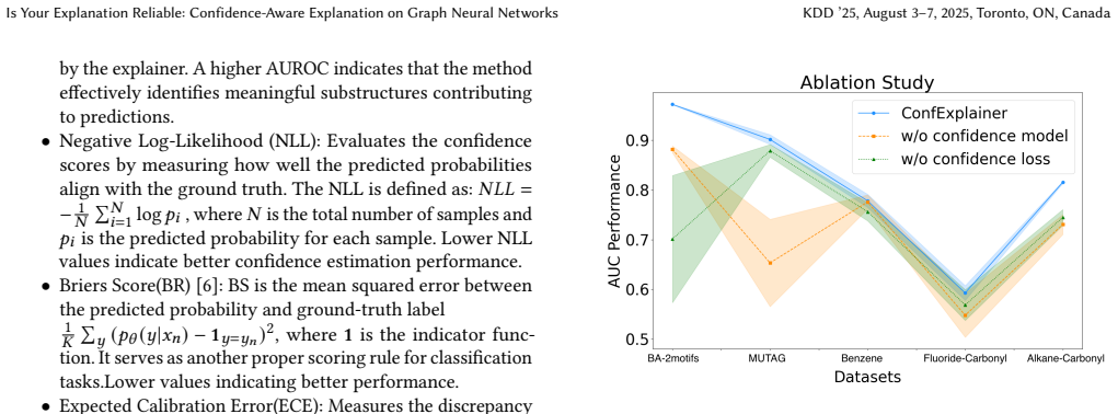
- Ablation results indicate that both the confidence module and the confidence loss contribute to explanation quality, not just to the confidence estimates themselves.
Reading between the lines
- A natural deployment use the paper does not develop: the confidence score can serve as a rejection rule, sending low-confidence explanations to human review or abstention in high-stakes settings.
- The equivalence argument suggests a further hypothesis the paper does not test: if the confidence weights are constrained to be sparse or structure-aware, the confidence matrix itself could double as a secondary, harder explanation mask.
- The out-of-distribution evaluation is performed by adding noise to node features; a stricter stress test would shift the label-relevant motif itself, which is exactly the regime where the paper concedes its central conditional-independence condition could fail.
- Because the confidence loss is supervised with true labels during training, the framework's calibration in a fully unsupervised deployment domain remains an open question that the experiments do not directly measure.
Editorial analysis
A structured set of objections, weighed in public.
Referee Report
Summary. The paper introduces ConfExplainer, a post-hoc instance-level explainer for GNNs that augments the graph information bottleneck (GIB) objective with a confidence scoring module (GIB-CC). The explanation subgraph is combined with Gaussian noise weighted by a learned confidence matrix, and a joint loss combines a GIB loss with a confidence loss. The authors claim that GIB-CC is equivalent to vanilla GIB (Property 1), report improved explanation AUC on four of five benchmark datasets, and present evidence that the learned confidence scores decrease when input noise is injected, indicating better calibration than baseline explainers.
Significance. If the central claims were correct, the paper would address a real gap: post-hoc GNN explainers generally do not provide a calibrated reliability score for their explanations, and a confidence-aware training objective that provably maintains GIB equivalence would be valuable. The authors also provide a public code repository and a linear-time confidence module, which are strengths. However, the theoretical equivalence rests on an invalid information identity and a circular conditional-independence assumption, and the confidence loss in Eq. (9) has an inverted sign. These issues undermine the claimed foundation and the interpretation of the experiments. The reported confidence-calibration numbers, including near-zero BR/ECE values in Table 2, are internally inconsistent, so the significance of the contribution is not currently established.
major comments (4)
- [4.1.2, Eq. (4)] The identity H(Y|G~)=H(Y|G')+I(C,Gr;Y|G') is not a valid decomposition of conditional entropy. For X=(G',C,Gr) and G~=phi(X), the correct identity is H(Y|G~)=H(Y|X)+I(Y;X|G~), while H(Y|G')=H(Y|X)+I(Y;C,Gr|G'). Hence H(Y|G~)=H(Y|G')-I(Y;C,Gr|G')+I(Y;X|G~). Even under the assumed condition I(C,Gr;Y|G')=0, the non-negative term I(Y;X|G~) need not vanish, so the claimed equality H(Y|G~)=H(Y|G') and Property 1 are not established by the given argument.
- [4.1.1 and Appendix B] The constraint I(C,Gr;Y|G')=0 in Eq. (2) is exactly the condition needed for the claimed equivalence, but its justification is circular: Appendix B derives it from the vanilla GIB optimality condition I(Y;G|G')=0, which is the property the optimization is supposed to achieve rather than a fact available during training. The paper itself concedes in Appendix B that the condition may fail under severe OOD shifts. Since the central theoretical claim depends on this equality, treating it as an assumption narrows the stated scope of the method, and it cannot be used to prove Property 1 without additional evidence that the condition actually holds for the learned G'.
- [4.2.2, Eq. (9)] The confidence loss has the wrong sign relative to its stated purpose. With M_tp=+1 for correct predictions and -1 for incorrect ones, the per-sample term is M_tp,i * C_i * (y~_i - y_i)^2. For hard-label predictions the squared error is 0 on correct samples and 1 on incorrect samples, so minimizing L_C drives C_i down for correct samples and up for incorrect samples; with soft targets the same inversion holds for samples with sufficiently small squared error. This directly contradicts the sentence following Eq. (9) and means the training signal does not encourage confidence to track explanation quality. The empirical confidence results in Figure 3 therefore lack support from the stated objective.
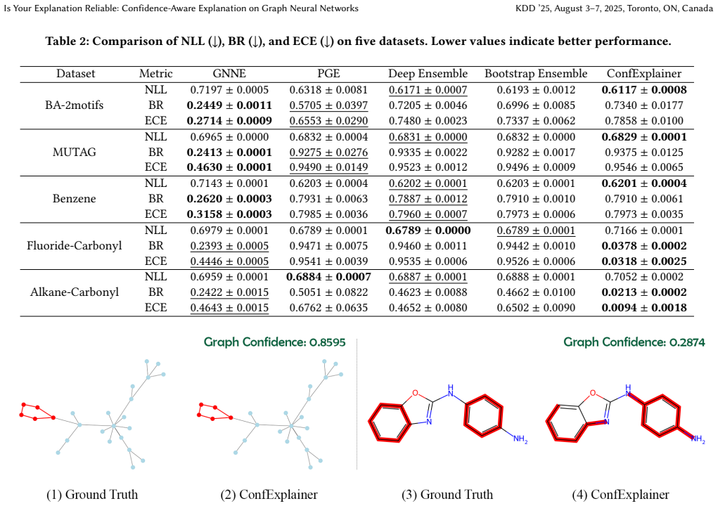
- [5.3 and Appendix D] The confidence evaluation is underspecified and internally inconsistent. The paper never defines how per-edge confidence scores C_ij are aggregated into the graph-level confidence used to compute NLL, BR, and ECE, and the formulas in Appendix D refer to predicted probabilities p_i without connecting them to the confidence matrix C. Moreover, Table 2 reports BR=0.0378 and ECE=0.0318 for ConfExplainer on Fluoride-Carbonyl while NLL=0.7166 (worse than baselines); such a combination is not attainable by any proper scoring rule and suggests that the quantity being evaluated differs from the one defined. Without a precise and consistent definition, the calibration claims in Section 5.3 cannot be assessed.
minor comments (6)
- [3.1] The phrase 'important typologies' should likely be 'important topologies' or 'important substructures.'
- [4.3] The complexity analysis contains an unmatched parenthesis and inconsistent symbols (|D_e|, D_n, E_n); please rewrite it with consistent notation and complete expressions.
- [5.1.1] BA-2motifs is described as a node-classification dataset, but the experimental setup in Table 1 reports graph-level classification results; clarify the task and how the ground-truth explanations are defined.
- [Figure 3] The x-axis is described as noise level epsilon in [0,1] plotted on a log scale, but log scale is not defined at zero; specify the actual plotted values or use a linear scale with a small offset.
- [Appendix D] The Brier score formula has mismatched indices and appears to miss a normalization factor; also 'Briers Score' should be 'Brier Score.'
- [Eq. (2)] The text 'while (1-C)⊙G_r' appears to be a typo for 'where (1-C)⊙G_r.'
Circularity Check
GIB-CC equivalence is imposed by constraint, and Eq. (9) inverts the claimed confidence-reliability link.
-
self definitional
[Section 4.1.2, Eqs. (2)-(5), Property 1]
"Given G_r as an independent sampled graph noise and C as an extrinsic generated score, we have I(C,G_r;Y|G')=0. A detailed illustration could be found in Appendix B. Therefore, we obtain: H(Y|\tilde G)=H(Y|G'), (5) which ensures that our framework, with the confidence-aware formulation, maintains equivalence with the original GIB formulation."
Eq. (2) imposes the constraint I(C,G_r;Y|G')=0, and Eqs. (3)-(5) then substitute that same constraint to conclude H(Y|\tilde G)=H(Y|G'). Consequently I(Y,\tilde G)=I(Y,G') and the objective in Eq. (2) is exactly Eq. (1). Property 1 is therefore not an independent result but a restatement of the assumption that cancels the newly introduced term; the 'generalized' objective contributes no mutual-information content beyond vanilla GIB, and the confidence mechanism is later supplied only through the separate, ungrounded loss in Eq. (9).
-
other
[Section 4.2.2, Eqs. (8)-(9)]
"M_tp(\tilde y,y)= (1, if \tilde y is correctly classified, -1, otherwise.) (8) Using this mask, our final confidence loss is written as: L_C = \beta \sum M_{tp,i}(C_i*(\tilde y_i-y)^2)/N ... This encourages the model to assign high confidence to correct explanations and low confidence to uncertain ones."
Under Eqs. (8)-(9), a correct hard-label prediction has (\tilde y_i-y_i)^2=0, so the loss contributes no C_i-dependent term and gives no gradient. For an incorrect hard-label prediction, M_{tp,i}=-1 and the squared term is positive, making the contribution -C_i; minimizing L_C therefore drives C_i upward. The equation as written rewards high confidence on wrong explanations and is silent on correct ones, which is the opposite of the sentence immediately following Eq. (9). The central claim that the confidence score reflects explanation reliability is thus not a consequence of the stated objective: confidence is trained as an inverted function of the explainer's own prediction error, and the reported OOD confidence decrease in Fig. 3 is not entailed by this loss.
full rationale
The only genuinely circular step in the derivation chain is Property 1: the GIB-CC objective is shown to equal vanilla GIB by invoking the very constraint that makes the new confidence term vanish, so the theoretical novelty reduces to a restatement of the paper's own equations. Separately, the confidence loss in Eq. (9) is internally contradictory: for incorrect hard-label predictions it simplifies to -C_i and pushes confidence up, while for correct predictions it provides no signal, directly inverting the stated principle that confidence should be high for reliable explanations and low for unreliable ones. This is a correctness/sign problem rather than a classical circular fit, but it breaks the claimed derivation from the loss to the measured OOD calibration behavior. The fidelity improvements in Table 1 are empirical and not themselves circular, and the paper does not rely on a load-bearing self-citation or an imported uniqueness theorem; for that reason the score is 6 rather than 8-10, reflecting partial circularity in the central theoretical claim and a contradictory training signal for the central confidence claim.
Assumptions & free parameters
free parameters (3)
- λ (confidence loss weight) =
100 (selected from {0.001, 0.01, 0.1, 1, 10, 100, 1000})
- β (confidence loss scale) =
Not reported
- α (GIB balancing coefficient) =
0.3 (inferred from config)
assumptions (3)
- domain assumption I(C,Gr;Y|G')=0
- standard math Standard mutual information identities
- domain assumption Ground-truth explanations are available for training/evaluation
Cite this review
Pith. "Pith review of Is Your Explanation Reliable: Confidence-Aware Explanation on Graph Neural Networks." pith.science (2026). https://pith.science/paper/O6BJR7TD
@misc{pith2026250600437,
  author       = {Pith},
  title        = {Pith review of: Is Your Explanation Reliable: Confidence-Aware Explanation on Graph Neural Networks},
  year         = {2026},
  howpublished = {\url{https://pith.science/paper/O6BJR7TD}},
  note         = {Machine review of arXiv:2506.00437}
}
read the original abstract
Explaining Graph Neural Networks (GNNs) has garnered significant attention due to the need for interpretability, enabling users to understand the behavior of these black-box models better and extract valuable insights from their predictions. While numerous post-hoc instance-level explanation methods have been proposed to interpret GNN predictions, the reliability of these explanations remains uncertain, particularly in the out-of-distribution or unknown test datasets. In this paper, we address this challenge by introducing an explainer framework with the confidence scoring module ( ConfExplainer), grounded in theoretical principle, which is generalized graph information bottleneck with confidence constraint (GIB-CC), that quantifies the reliability of generated explanations. Experimental results demonstrate the superiority of our approach, highlighting the effectiveness of the confidence score in enhancing the trustworthiness and robustness of GNN explanations.
Figures


Figures from the paper (4 more)


Reference graph
Works this paper leans on
-
[1]
Moloud Abdar, Farhad Pourpanah, Sadiq Hussain, Dana Rezazadegan, Li Liu, Mo- hammad Ghavamzadeh, Paul Fieguth, Xiaochun Cao, Abbas Khosravi, U Rajendra Acharya, et al. 2021. A review of uncertainty quantification in deep learning: Techniques, applications and challenges. Information fusion 76 (2021), 243–297
work page 2021
-
[2]
Chirag Agarwal, Owen Queen, Himabindu Lakkaraju, and Marinka Zitnik. 2023. Evaluating explainability for graph neural networks. Scientific Data 10, 1 (2023), 144
2023
-
[3]
Réka Albert and Albert-László Barabási. 2002. Statistical mechanics of complex networks. Reviews of modern physics 74, 1 (2002), 47
work page 2002
-
[4]
Federico Baldassarre and Hossein Azizpour. 2019. Explainability Techniques for Graph Convolutional Networks
work page 2019
-
[5]
Muhammed Fatih Balın, Abubakar Abid, and James Zou. 2019. Concrete au- toencoders: Differentiable feature selection and reconstruction. In International conference on machine learning . PMLR, 444–453
work page 2019
-
[6]
Glenn W Brier. 1950. Verification of forecasts expressed in terms of probability. Monthly weather review 78, 1 (1950), 1–3
1950
-
[7]
Zhuomin Chen, Jiaxing Zhang, Jingchao Ni, Xiaoting Li, Yuchen Bian, Md Mezbahul Islam, Ananda Mondal, Hua Wei, and Dongsheng Luo. 2024. Generating In-Distribution Proxy Graphs for Explaining Graph Neural Net- works. In Forty-first International Conference on Machine Learning . https: //openreview.net/forum?id=ohG9bVMs5j
work page 2024
-
[8]
Enyan Dai and Suhang Wang. 2021. Towards Self-Explainable Graph Neural Network
work page 2021
Show all 43 references
-
[9]
Enyan Dai, Tianxiang Zhao, Huaisheng Zhu, Junjie Xu, Zhimeng Guo, Hui Liu, Jiliang Tang, and Suhang Wang. 2024. A comprehensive survey on trustworthy graph neural networks: Privacy, robustness, fairness, and explainability.Machine Intelligence Research 21, 6 (2024), 1011–1061
2024
-
[10]
Vincenzo Marco De Luca, Antonio Longa, Pietro Lio, and Andrea Passerini. [n. d.]. xAI-Drop: Don’t use what you cannot explain. In The Third Learning on Graphs Conference
-
[11]
Wenqi Fan, Yao Ma, Qing Li, Yuan He, Eric Zhao, Jiliang Tang, and Dawei Yin
-
[12]
Jeroen Kazius, Ross McGuire, and Roberta Bursi. 2005. Derivation and validation of toxicophores for mutagenicity prediction. Journal of medicinal chemistry 48, 1 (2005), 312–320
2005
-
[13]
Balaji Lakshminarayanan, Alexander Pritzel, and Charles Blundell. 2017. Simple and scalable predictive uncertainty estimation using deep ensembles. Advances in neural information processing systems 30 (2017)
2017
-
[14]
Trevino, Jiliang Tang, and Huan Liu
Jundong Li, Kewei Cheng, Suhang Wang, Fred Morstatter, Robert P. Trevino, Jiliang Tang, and Huan Liu. 2017. Feature Selection: A Data Perspective. ACM Comput. Surv. 50, 6, Article 94 (dec 2017), 45 pages. https://doi.org/10.1145/ 3136625
2017
-
[15]
Mengzhang Li and Zhanxing Zhu. 2021. Spatial-Temporal Fusion Graph Neural Networks for Traffic Flow Forecasting. Proceedings of the AAAI Conference on Artificial Intelligence 35, 5 (May 2021), 4189–4196
2021
-
[16]
Yang Li, Buyue Qian, Xianli Zhang, and Hui Liu. 2020. Graph neural network- based diagnosis prediction. Big data 8, 5 (2020), 379–390
2020
-
[17]
Dongsheng Luo, Wei Cheng, Dongkuan Xu, Wenchao Yu, Bo Zong, Haifeng Chen, and Xiang Zhang. 2020. Parameterized explainer for graph neural network. Advances in neural information processing systems 33 (2020), 19620–19631
2020
-
[18]
Siqi Miao, Mia Liu, and Pan Li. 2022. Interpretable and generalizable graph learn- ing via stochastic attention mechanism. In International Conference on Machine Learning. PMLR, 15524–15543
2022
-
[19]
Shengjie Min, Zhan Gao, Jing Peng, Liang Wang, Ke Qin, and Bo Fang. 2021. STGSN — A Spatial–Temporal Graph Neural Network framework for time- evolving social networks. Knowledge-Based Systems 214 (2021), 106746
2021
-
[20]
Owen Queen. 2022. GraphXAI. https://doi.org/10.7910/DVN/KULOS8
2022 doi
-
[21]
Benjamin Sanchez-Lengeling, Jennifer Wei, Brian Lee, Emily Reif, Peter Wang, Wesley Qian, Kevin McCloskey, Lucy Colwell, and Alexander Wiltschko. 2020. Evaluating attribution for graph neural networks. Advances in neural information processing systems 33 (2020), 5898–5910
2020
-
[22]
Caihua Shan, Yifei Shen, Yao Zhang, Xiang Li, and Dongsheng Li. 2021. Reinforce- ment Learning Enhanced Explainer for Graph Neural Networks. In Advances in Neural Information Processing Systems , A. Beygelzimer, Y. Dauphin, P. Liang, and J. Wortman Vaughan (Eds.). https://open...
2021
-
[23]
Indro Spinelli, Simone Scardapane, and Aurelio Uncini. 2022. A meta-learning approach for training explainable graph neural networks. IEEE Transactions on Neural Networks and Learning Systems (2022)
2022
-
[24]
Ronast Subedi, Lu Wei, Wenhan Gao, Shayok Chakraborty, and Yi Liu. 2024. Empowering Active Learning for 3D Molecular Graphs with Geometric Graph Isomorphism. In Advances in Neural Information Processing Systems, A. Globerson, L. Mackey, D. Belgrave, A. Fan, U. Paquet, J. Tomcz...
2024
-
[25]
Fangxin Wang, Yuqing Liu, Kay Liu, Yibo Wang, Sourav Medya, and Philip S Yu. 2024. Uncertainty in Graph Neural Networks: A Survey. arXiv preprint arXiv:2403.07185 (2024)
2024 arXiv
-
[26]
Xiaoyang Wang, Yao Ma, Yiqi Wang, Wei Jin, Xin Wang, Jiliang Tang, Caiyan Jia, and Jian Yu. 2020. Traffic Flow Prediction via Spatial Temporal Graph Neural Network. In Proceedings of The Web Conference 2020 (Taipei, Taiwan) (WWW ’20). Association for Computing Machinery, New Y...
2020
-
[27]
Xiang Wang, Yingxin Wu, An Zhang, Xiangnan He, and Tat-seng Chua. 2021. Causal screening to interpret graph neural networks. (2021)
2021
-
[28]
Tailin Wu, Hongyu Ren, Pan Li, and Jure Leskovec. 2020. Graph information bottleneck. Advances in Neural Information Processing Systems 33 (2020), 20437– 20448
2020
-
[29]
Zonghan Wu, Shirui Pan, Guodong Long, Jing Jiang, and Chengqi Zhang. 2019. Graph Wavenet for Deep Spatial-Temporal Graph Modeling. In Proceedings of the 28th International Joint Conference on Artificial Intelligence (Macao, China) (IJCAI’19). AAAI Press, 1907–1913
2019
-
[30]
Liu Xufeng, Luo Dongsheng, Gao Wenhan, and Liu Yi. 2024. 3DGraphX: Explain- ing 3D Molecular Graph Models via Incorporating Chemical Priors. InProceedings of the 31th ACM SIGKDD Conference on Knowledge Discovery and Data Mining
2024
-
[31]
Zhitao Ying, Dylan Bourgeois, Jiaxuan You, Marinka Zitnik, and Jure Leskovec
-
[32]
Bing Yu, Haoteng Yin, and Zhanxing Zhu. 2018. Spatio-Temporal Graph Con- volutional Networks: A Deep Learning Framework for Traffic Forecasting. In Proceedings of the Twenty-Seventh International Joint Conference on Artificial Intelligence, IJCAI-18. International Joint Confer...
2018
- [33]
-
[34]
Hao Yuan, Haiyang Yu, Jie Wang, Kang Li, and Shuiwang Ji. 2021. On explain- ability of graph neural networks via subgraph explorations. In International Conference on Machine Learning . PMLR, 12241–12252
2021
-
[35]
Junchi Yu, Tingyang Xu, Yu Rong, Yatao Bian, Junzhou Huang, and Ran He
-
[36]
Jiaxing Zhang, Jiayi Liu, Dongsheng Luo, Jennifer Neville, and Hua Wei. 2024. LLMExplainer: Large Language Model based Bayesian Inference for Graph Ex- planation Generation
2024
-
[37]
Jiaxing Zhang, Dongsheng Luo, and Hua Wei. 2023. MixupExplainer: Gener- alizing Explanations for Graph Neural Networks with Data Augmentation. In Proceedings of 29th ACM SIGKDD Conference on Knowledge Discovery and Data Mining (SIGKDD)
2023
-
[38]
Jiaxing Zhang, Zhuomin Chen, hao mei, Longchao Da, Dongsheng Luo, and Hua Wei. 2024. RegExplainer: Generating Explanations for Graph Neural Networks in Regression Tasks. In Advances in Neural Information Processing Systems , Vol. 37. Curran Associates, Inc., 79282–79306
2024
-
[39]
Jie Zhou, Ganqu Cui, Shengding Hu, Zhengyan Zhang, Cheng Yang, Zhiyuan Liu, Lifeng Wang, Changcheng Li, and Maosong Sun. 2020. Graph neural networks: A review of methods and applications. AI open 1 (2020), 57–81. KDD ’25, August 3–7, 2025, Toronto, ON, Canada Zhang et al. A No...
2020
-
[41]
Xin Zhang, Zhen Xu, Yue Liu, Mengfang Sun, Tong Zhou, and Wenying Sun. 2024. Robust Graph Neural Networks for Stability Analysis in Dynamic Networks. In 2024 3rd International Conference on Cloud Computing, Big Data Application and Software Engineering (CBASE). IEEE, 806–811
2024
-
[43]
The calibrated graph construction involves a weighted sum: ˜𝐺 = 𝐶⊙𝐺′+( 1−𝐶)⊙ 𝐺𝑟 , with complexityO(|𝐸|). 3. Total training cost per iteration is thus linear in the graph size: O(|𝐸|𝑑), consistent with prior works like PGExplainer. Table 4 compares wall-clock training time with...
2025
-
[2019]
Graph Neural Networks for Social Recommendation
-
[2020]
arXiv preprint arXiv:2010.05563 (2020)
Graph information bottleneck for subgraph recognition. arXiv preprint arXiv:2010.05563 (2020)
2020 arXiv
Reviewed August 7, 2026 · model on record in the stance chip above.
Discussion (0). Sign in to comment.