REVIEW 4 major objections 6 minor 80 references
Flying Co-Stereo: Enabling Long-Range Aerial Dense Mapping via Collaborative Stereo Vision of Dynamic-Baseline
T0 review · 4 major / 6 minor · reviewed 2026-08-07 · deepseek-v4-flash
Pith's one-line read Two cooperating drones form a wide-baseline stereo pair whose sparse triangulated landmarks rescale monocular depth estimates, yielding dense metric maps out to 70 meters with 2.3-9.7% relative error.
desk verdict A real two-UAV dynamic-baseline stereo system with solid engineering and a plausible but not fully secured 70 m dense-mapping claim; worth peer review with requests for stronger evaluation. read the letter →
The pith
A machine-rendered reading of the paper's core claim, the machinery that carries it, and where it could break.
The reading
What carries the argument
The load-bearing object is the exponential depth-fitting model in Eq. (13): a curve $\hat z = a\exp(b(\tilde d - c)) + d$ mapping the monocular network's up-to-scale depth $\tilde d$ to metric depth $\hat z$, with four parameters fitted from only 60-200 sparse landmarks using Ceres. This single global curve is what converts near-field VIO landmarks and long-range collaboratively triangulated landmarks into a full 640x480 dense metric depth image. Around it, the system stacks the DS-VIRE sliding-window estimator, which fuses visual PnP from infrared markers with IMU and UWB range factors and uses a bidirectional view differential for yaw, and the GP-SS hybrid, which uses periodic SuperPoint-SuperGlue matching as guidance and LK optical flow as continuous prediction. The machinery's job is to supply the sparse metric anchor points at long range and the accurate relative baseline that makes their triangulation stable.
What would settle it
Use a held-out outdoor scene with lidar ground truth: fit the four exponential parameters using only landmarks in the 30-50 m band, then compute per-pixel relative depth error on pixels beyond 70 m or in featureless regions; if those errors exceed the reported 2.3-9.7% band, or if the residual grows systematically with depth, the global-exponential assumption is false.
Extended reading notes
Core claim
Flying Co-Stereo's central claim is that a dynamic cross-agent baseline of 2-5 m between two UAVs turns their forward cameras into a wide-baseline stereo rig whose long-range parallax supports metric triangulation of distant co-visible landmarks, and that these landmarks are enough to convert an up-to-scale monocular depth prediction from DepthAnythingV2 into a dense metric depth map via a four-parameter exponential fit. The reported result is dense 3D mapping to 70 m with 2.3-9.7% relative error, with the wide-baseline configuration beating a 95 mm fixed stereo camera by up to 350% in range and 450% in coverage. The argument is carried by three coupled modules: the dual-spectrum visual-inertial-ranging estimator DS-VIRE for the time-varying baseline, the guidance-prediction feature association GP-SS for persistent co-visible points across dynamic viewpoints, and the exponential sparse-to-dense fitting that supplies the metric scale.
Load-bearing premise
The whole dense map is produced by one four-parameter exponential curve fitted to only 60-200 sparse landmarks, so the accuracy claim holds only if the monocular depth network's up-to-scale depth is globally exponential across every pixel of the 640x480 image, including far regions with no landmarks.
Editorial extensions
If this is right
- Map range jumps from about 20 m to 70 m while the payload stays two lightweight camera-IMU-UWB drones, with no lidar.
- Coverage area of the dense map is 331-450% larger than the onboard RealSense D455 stereo in the three outdoor test scenes.
- Exponential fitting beats linear and quadratic alternatives consistently, cutting unidirectional Chamfer error by an average of 67% versus linear and 55% versus quadratic.
- Real-time operation on a Jetson Xavier NX is feasible: GP-SS sustains near-30 Hz feature association instead of 13 Hz for full SuperGlue, while DS-MVDT keeps tracking the neighbor drone in 96-99% of frames across challenging outdoor scenes.
- A baseline of 2-4 m balances triangulation stability against baseline-estimation error, with yaw estimation reaching 0.214 degrees mean absolute error.
Reading between the lines
- Editorial inference: if the exponential map between up-to-scale and metric depth is a property of the monocular network rather than of these particular scenes, the same sparse-to-dense recipe transfers to any future depth predictor by refitting the four parameters per frame.
- Editorial inference: the measured baseline-length trade-off implies an active baseline controller could widen the drone separation when the scene is far and narrow it when the scene is near, a line the paper itself lists as future work.
- Editorial inference: a held-out per-pixel test against lidar on regions without co-visible or VIO landmarks would reveal whether the global exponential fit, rather than the landmarks themselves, is carrying the 50-70 m far-field accuracy.
- Editorial inference: stringing pairs so each drone tracks its predecessor and guides its successor would extend the moving baseline into a swarm-scale network, with coverage growing linearly with chain length; the paper names this as a future architecture.
Editorial analysis
A structured set of objections, weighed in public.
Referee Report
Summary. The paper proposes Flying Co-Stereo, a collaborative stereo mapping system in which two UAVs carrying forward-facing cameras form a wide, dynamic baseline. The system estimates the time-varying baseline with a dual-spectrum visual-inertial-ranging estimator (DS-VIRE), associates co-visible features across agents with a guidance-prediction SuperPoint/SuperGlue plus optical-flow scheme (GP-SS), and produces dense metric depth by exponentially fitting sparse triangulated landmarks to the up-to-scale depth of DepthAnythingV2 (Eq. 13). Experiments report baseline estimation MAE of 0.013 m and yaw MAE of 0.214 deg indoors, robust IR-marker tracking outdoors, and dense mapping up to 70 m with relative errors of 2.3% to 9.7% computed via a unidirectional Chamfer distance against R3LIVE ground truth, plus comparisons against a fixed-baseline RealSense stereo and two MVS methods.
Significance. If the central claim holds, the system is a meaningful step toward lightweight, long-range dense mapping for UAV swarms without LiDAR. The paper's strengths include real dual-UAV flight experiments, external motion-capture and R3LIVE ground truth, a concrete sparse-to-dense pipeline that goes beyond the linear fitting used in AB-VINS, and a clear analysis of triangulation stability versus baseline length. However, the headline dense-mapping accuracy rests on an evaluation design that does not yet validate every pixel of the reconstructed depth image, and the experimental basis is limited to very few frames per scene. These issues are fixable and do not invalidate the system concept, but they prevent the reported error numbers from being accepted at face value.
major comments (4)
- [Sec. VII-F, Eq. (17)] The dense-mapping accuracy metric uCD(P→G) is unidirectional: for each predicted point it queries only the nearest ground-truth point, so missing predicted geometry or arbitrarily sparse coverage in a depth band does not increase the error. The abstract and conclusion claim 2.3%–9.7% relative error and 70 m dense mapping based on this metric. Please also report a bidirectional Chamfer distance or a completeness/coverage metric (e.g., fraction of ground-truth points within a tolerance), and report per-pixel depth errors on the dense depth images rather than only on resampled predicted clouds.
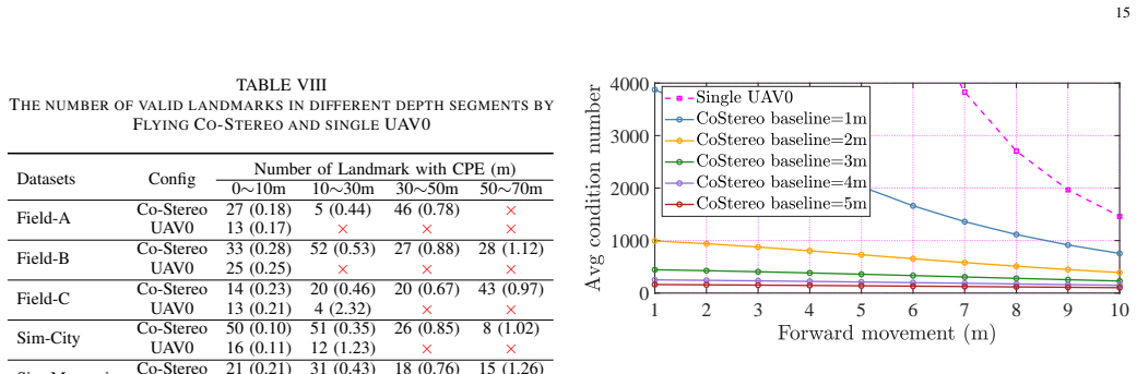
- [Sec. VI-B, Eq. (13) and Sec. VII-F, Table IX] The four-parameter exponential transform is fit from only 60–200 sparse landmarks, and the evaluation does not separate landmark-supervised pixels from held-out pixels. As written, the reported depth-segment errors could reflect accuracy only near the sparse landmarks or in depth regimes where the landmarks are dense, not across the full 640×480 image out to 70 m. Please add a held-out validation protocol: fit the transform on one subset of landmarks (e.g., by depth band or spatial region) and evaluate the dense depth on the remaining landmarks or, better, on per-pixel R3LIVE depth, reporting errors per depth segment and per scene.
- [Sec. VII, Table VII and Sec. VII-F] The real-world dense-mapping evaluation uses only 4 camera frames per UAV per scene and a single flight per scene, with no repeated trials or error bars. For a claim of up to 70 m dense mapping and 331–450% coverage improvement, the evaluation should include longer sequences or repeated flights so that the reported uCD values and coverage areas are not artifacts of a single, short snippet. Please report means and variances over multiple runs or, failing that, explicitly state the single-run nature as a limitation.
- [Sec. VII-F, Table IX and Sec. VI-B] The paper does not state how the predicted point cloud P in Eq. (17) is generated from the dense depth map: whether all depth-image pixels are resampled, whether a depth threshold or confidence mask is applied, and how many points fall into each of the 0–10 m, 10–30 m, 30–50 m, and 50–70 m segments. Without this information, the per-segment relative errors in Table IX cannot be interpreted as dense reconstruction accuracy; they may reflect only a small subset of the image. Please specify the point-cloud generation procedure and report per-segment point counts and completeness.
minor comments (6)
- [Sec. IV-B, Eq. (3)] The visual residual in Eq. (3) is written as a two-row vector with a zero second row, but the context suggests it should be a 3-D position residual; please clarify the notation or remove the spurious zero component.
- [Sec. VI-A] The condition-number threshold used to discard poorly conditioned triangulations is never given; please report the actual threshold or the range used in the experiments.
- [Sec. VII-D, Table VI] The GP-SS total run-time is reported as "7.4/82.4 ms", which is ambiguous; please clarify which number is the LK-flow-only cost and which is the periodic SuperPoint/SuperGlue cost.
- [Sec. VII-F, Table IX] The relative error is defined as the ratio of uCD to the average depth of the segment, but the average depth values are not reported; please state them explicitly so the reader can verify the percentages.
- [Sec. VII and References] No code or data availability statement is provided; releasing the datasets and implementation would substantially strengthen reproducibility, especially given the small number of evaluation frames.
- [Throughout] There are typographical and formatting issues, including "V oxblox" in the Fig. 22 caption, "moshed WiFi" in Sec. VII-B, and inconsistent capitalization of "UAV" across the text; these should be cleaned up.
Circularity Check
No significant circularity: the dense mapping result is evaluated against external R3LIVE ground truth, and the exponential fit (Eq. 13) is a per-frame scaling model whose inputs are sparse landmarks, not the reported dense-map metric.
full rationale
The paper's derivation chain is self-contained in the sense required by the circularity analysis. Baseline estimation (DS-VIRE, Eqs. 1-7) fuses independent IMU, UWB, and infrared-marker observations; feature association (GP-SS) is a real engineering contribution; collaborative triangulation (Eqs. 8-12) produces metric sparse landmarks from multi-view observations; and the sparse-to-dense step (Eq. 13) fits four parameters (a, b, c, d) of an exponential functional form to those sparse landmarks, then applies the fitted transform to the entire monocular depth image. This is a fitted-parameter-to-dense-prediction scheme, but it is not circular: the prediction target is the dense depth map, which is not defined as the fitted landmarks, and the reported 2.3%-9.7% relative errors are computed in Table IX against external R3LIVE ground truth using the uCD metric (Eq. 17), not against the landmarks used in the fit. The exponential form is chosen based on an observed depth-distribution pattern (Fig. 7b) and is empirically benchmarked against linear and quadratic fitting; this is in-sample model selection rather than a circular reduction. No load-bearing uniqueness theorem is imported from the authors' prior work, and the self-citations appearing in the related-work section (e.g., [17], [53], [66]) are contextual and do not justify the central claim. The acknowledged communication-interruption limitation is a scope caveat, not a circular step. Any concerns about per-pixel generalization, unidirectional Chamfer metric, or the small number of evaluation frames are correctness-risk issues, not circularity.
Assumptions & free parameters
free parameters (2)
- exponential fitting parameters a, b, c, d (Eq. 13) =
not reported; optimized per frame on 60-200 sparse landmarks via Ceres
- condition number threshold for landmark acceptance (Sec VI-A) =
not reported
assumptions (5)
- domain assumption R3LIVE LiDAR-inertial reconstruction is accurate ground truth at 10-70 m depth in open outdoor scenes.
- domain assumption DepthAnythingV2's relative depth output is globally related to metric depth by a single exponential transform per frame.
- standard math PnP, IMU preintegration, and UWB residual models are unbiased and correctly fused in the sliding window.
- ad hoc to paper Bidirectional yaw estimate Eq (7) treats a bright IR marker as a proxy for the side camera center and assumes near-hovering roll/pitch, with a level-frame correction.
- domain assumption The UAV formation stays within 5 m with low-latency WiFi; mapping pauses during communication interruptions.
Cite this review
Pith. "Pith review of Flying Co-Stereo: Enabling Long-Range Aerial Dense Mapping via Collaborative Stereo Vision of Dynamic-Baseline." pith.science (2026). https://pith.science/paper/5NWY5ZCM
@misc{pith2026250600546,
  author       = {Pith},
  title        = {Pith review of: Flying Co-Stereo: Enabling Long-Range Aerial Dense Mapping via Collaborative Stereo Vision of Dynamic-Baseline},
  year         = {2026},
  howpublished = {\url{https://pith.science/paper/5NWY5ZCM}},
  note         = {Machine review of arXiv:2506.00546}
}
read the original abstract
Lightweight long-range mapping is critical for safe navigation of UAV swarms in large-scale unknown environments. Traditional stereo vision systems with fixed short baselines face limited perception ranges. To address this, we propose Flying Co-Stereo, a cross-agent collaborative stereo vision system that leverages the wide-baseline spatial configuration of two UAVs for long-range dense mapping. Key innovations include: (1) a dual-spectrum visual-inertial-ranging estimator for robust baseline estimation; (2) a hybrid feature association strategy combining deep learning-based cross-agent matching and optical-flow-based intra-agent tracking; (3) A sparse-to-dense depth recovery scheme,refining dense monocular depth predictions using exponential fitting of long-range triangulated sparse landmarks for precise metric-scale mapping. Experiments demonstrate the Flying Co-Stereo system achieves dense 3D mapping up to 70 meters with 2.3%-9.7% relative error, outperforming conventional systems by up to 350% in depth range and 450% in coverage area. The project webpage: https://xingxingzuo.github.io/flying_co_stereo
Figures


Figures from the paper (20 more)




Reference graph
Works this paper leans on
-
[1]
Safety-assured high-speed navigation for mavs,
Y . Ren, F. Zhu, G. Lu, Y . Cai, L. Yin, F. Kong, J. Lin, N. Chen, and F. Zhang, “Safety-assured high-speed navigation for mavs,”Science Robotics, vol. 10, no. 98, p. eado6187, 2025
2025
-
[2]
Learning high-speed flight in the wild,
A. Loquercio, E. Kaufmann, R. Ranftl, M. M ¨uller, V . Koltun, and D. Scaramuzza, “Learning high-speed flight in the wild,”Science Robotics, vol. 6, no. 59, p. eabg5810, 2021
2021
-
[3]
Swarm of micro flying robots in the wild,
X. Zhou, X. Wen, Z. Wang, Y . Gao, H. Li, Q. Wang, T. Yang, H. Lu, Y . Cao, C. Xu, and F. Gao, “Swarm of micro flying robots in the wild,” Science Robotics, vol. 7, no. 66, p. eabm5954, 2022
work page 2022
-
[4]
Search and rescue under the forest canopy using multiple uavs,
Y . Tian, K. Liu, K. Ok, L. Tran, D. Allen, N. Roy, and J. P. How, “Search and rescue under the forest canopy using multiple uavs,”The International Journal of Robotics Research, vol. 39, no. 10-11, pp. 1201– 1221, 2020
2020
-
[5]
Lic-fusion: Lidar- inertial-camera odometry,
X. Zuo, P. Geneva, W. Lee, Y . Liu, and G. Huang, “Lic-fusion: Lidar- inertial-camera odometry,” inProc. IEEE/RSJ International Conference on Intelligent Robots and Systems, Macau, China, 2019, pp. 5848–5854
work page 2019
-
[6]
LIC-Fusion 2.0: LiDAR-inertial-camera odometry with sliding-window plane-feature tracking,
X. Zuo, Y . Yang, P. Geneva, J. Lv, Y . Liu, G. Huang, and M. Pollefeys, “LIC-Fusion 2.0: LiDAR-inertial-camera odometry with sliding-window plane-feature tracking,” inProc. IEEE/RSJ International Conference on Intelligent Robots and Systems, Las Vegas, NV , USA, 2020, pp. 5112– 5119
work page 2020
-
[7]
Clins: Continuous- time trajectory estimation for lidar-inertial system,
J. Lv, K. Hu, J. Xu, Y . Liu, X. Ma, and X. Zuo, “Clins: Continuous- time trajectory estimation for lidar-inertial system,” in2021 IEEE/RSJ International Conference on Intelligent Robots and Systems (IROS). IEEE, 2021, pp. 6657–6663
work page 2021
-
[8]
Viral-fusion: A visual-inertial-ranging-lidar sensor fusion approach,
T.-M. Nguyen, M. Cao, S. Yuan, Y . Lyu, T. H. Nguyen, and L. Xie, “Viral-fusion: A visual-inertial-ranging-lidar sensor fusion approach,” IEEE Transactions on Robotics, vol. 38, no. 2, pp. 958–977, 2021
work page 2021
Show all 80 references
-
[9]
Coco-LIC: Continuous-time tightly-coupled lidar-inertial-camera odometry using non-uniform b-spline,
X. Lang, C. Chen, K. Tang, Y . Ma, J. Lv, Y . Liu, and X. Zuo, “Coco-LIC: Continuous-time tightly-coupled lidar-inertial-camera odometry using non-uniform b-spline,”IEEE Robotics and Automation Letters, vol. 8, no. 11, pp. 7074–7081, 2023
2023
-
[10]
Gaussian-LIC: Real-time photo-realistic slam with gaussian splatting and lidar-inertial-camera fusion,
X. Lang, L. Li, C. Wu, C. Zhao, L. Liu, Y . Liu, J. Lv, and X. Zuo, “Gaussian-LIC: Real-time photo-realistic slam with gaussian splatting and lidar-inertial-camera fusion,” in2025 IEEE International Conference on Robotics and Automation (ICRA). IEEE, 2025
2025
-
[11]
Computa- tionally efficient trajectory planning for high speed obstacle avoidance of a quadrotor with active sensing,
G. Chen, D. Sun, W. Dong, X. Sheng, X. Zhu, and H. Ding, “Computa- tionally efficient trajectory planning for high speed obstacle avoidance of a quadrotor with active sensing,”IEEE Robotics and Automation Letters, vol. 6, no. 2, pp. 3365–3372, 2021
2021
-
[12]
An active sense and avoid system for flying robots in dynamic environments,
G. Chen, W. Dong, X. Sheng, X. Zhu, and H. Ding, “An active sense and avoid system for flying robots in dynamic environments,”IEEE/ASME Transactions on Mechatronics, vol. 26, no. 2, pp. 668–678, 2021
2021
-
[13]
Flexible trinocular: Non-rigid multi-camera-imu dense reconstruction for uav navigation and mapping,
T. Hinzmann, C. Cadena, J. Nieto, and R. Siegwart, “Flexible trinocular: Non-rigid multi-camera-imu dense reconstruction for uav navigation and mapping,” in2019 IEEE/RSJ International Conference on Intelligent Robots and Systems (IROS). IEEE, 2019, pp. 1137–1142
2019
-
[14]
Variable baseline/resolution stereo,
D. Gallup, J.-M. Frahm, P. Mordohai, and M. Pollefeys, “Variable baseline/resolution stereo,” in2008 IEEE conference on computer vision and pattern recognition. IEEE, 2008, pp. 1–8
2008
-
[15]
Collaborative stereo,
M. W. Achtelik, S. Weiss, M. Chli, F. Dellaerty, and R. Siegwart, “Collaborative stereo,” in2011 IEEE/RSJ International Conference on Intelligent Robots and Systems. IEEE, 2011, pp. 2242–2248
2011
-
[16]
Distributed variable-baseline stereo slam from two uavs,
M. Karrer and M. Chli, “Distributed variable-baseline stereo slam from two uavs,” in2021 IEEE International Conference on Robotics and Automation (ICRA). IEEE, 2021, pp. 82–88
2021
-
[17]
A collaborative stereo camera with two uavs for long-distance mapping of urban buildings,
Z. Wang and W. Dong, “A collaborative stereo camera with two uavs for long-distance mapping of urban buildings,” in2024 IEEE/RSJ International Conference on Intelligent Robots and Systems (IROS). IEEE, 2024, pp. 7944–7951
2024
-
[18]
Agile Formation Control of Drone Flocking Enhanced With Active Vision-Based Relative Localiza- tion,
P. Zhang, G. Chen, Y . Li, and W. Dong, “Agile Formation Control of Drone Flocking Enhanced With Active Vision-Based Relative Localiza- tion,”IEEE Robotics and Automation Letters, vol. 7, no. 3, pp. 6359– 6366, Jul. 2022
2022
-
[19]
Fiducial markers for pose estimation: Overview, appli- cations and experimental comparison of the artag, apriltag, aruco and stag markers,
M. Kalaitzakis, B. Cain, S. Carroll, A. Ambrosi, C. Whitehead, and N. Vitzilaios, “Fiducial markers for pose estimation: Overview, appli- cations and experimental comparison of the artag, apriltag, aruco and stag markers,”Journal of Intelligent&Robotic Systems, vol. 101, no. 4...
2021
-
[20]
Vision-based drone flocking in outdoor environments,
F. Schilling, F. Schiano, and D. Floreano, “Vision-based drone flocking in outdoor environments,”IEEE Robotics and Automation Letters, vol. 6, no. 2, pp. 2954–2961, 2021
2021
-
[21]
Vision-based multi-mav localization with anonymous relative measurements using coupled probabilistic data association filter,
T. Nguyen, K. Mohta, C. J. Taylor, and V . Kumar, “Vision-based multi-mav localization with anonymous relative measurements using coupled probabilistic data association filter,” in2020 IEEE International Conference on Robotics and Automation (ICRA). IEEE, 2020, pp. 3349–3355
2020
-
[22]
Tracking and Relative Localization of Drone Swarms With a Vision- Based Headset,
M. Pavliv, F. Schiano, C. Reardon, D. Floreano, and G. Loianno, “Tracking and Relative Localization of Drone Swarms With a Vision- Based Headset,”IEEE Robotics and Automation Letters, vol. 6, no. 2, pp. 1455–1462, 2021
2021
-
[23]
6- dof object pose from semantic keypoints,
G. Pavlakos, X. Zhou, A. Chan, K. G. Derpanis, and K. Daniilidis, “6- dof object pose from semantic keypoints,” in2017 IEEE international conference on robotics and automation (ICRA). IEEE, 2017, pp. 2011– 2018
2017
-
[24]
Vi-rpe: Visual-inertial relative pose estimation for aerial vehicles,
L. Teixeira, F. Maffra, M. Moos, and M. Chli, “Vi-rpe: Visual-inertial relative pose estimation for aerial vehicles,”IEEE Robotics and Automa- tion Letters, vol. 3, no. 4, pp. 2770–2777, 2018
2018
-
[25]
Robust Visual Positioning of the UA V for the Under Bridge Inspection With a Ground Guided Vehicle,
Z. Wang, S. Liu, G. Chen, and W. Dong, “Robust Visual Positioning of the UA V for the Under Bridge Inspection With a Ground Guided Vehicle,”IEEE Transactions on Instrumentation and Measurement, vol. 71, pp. 1–10, 2022
2022
-
[26]
Uvdar system for visual relative localization with application to leader–follower formations of multirotor uavs,
V . Walter, N. Staub, A. Franchi, and M. Saska, “Uvdar system for visual relative localization with application to leader–follower formations of multirotor uavs,”IEEE Robotics and Automation Letters, vol. 4, no. 3, pp. 2637–2644, 2019
2019
-
[27]
Crepes: Cooperative relative pose estimation system,
Z. Xun, J. Huang, Z. Li, Z. Ying, Y . Wang, C. Xu, F. Gao, and Y . Cao, “Crepes: Cooperative relative pose estimation system,” in2023 IEEE/RSJ International Conference on Intelligent Robots and Systems (IROS). IEEE, 2023, pp. 5274–5281
2023
-
[28]
Decentralized visual- inertial-uwb fusion for relative state estimation of aerial swarm,
H. Xu, L. Wang, Y . Zhang, K. Qiu, and S. Shen, “Decentralized visual- inertial-uwb fusion for relative state estimation of aerial swarm,” in 2020 IEEE international conference on robotics and automation (ICRA). IEEE, 2020, pp. 8776–8782
2020
-
[29]
Omni-swarm: A decentralized omnidirectional visual–inertial– uwb state estimation system for aerial swarms,
H. Xu, Y . Zhang, B. Zhou, L. Wang, X. Yao, G. Meng, and S. Shen, “Omni-swarm: A decentralized omnidirectional visual–inertial– uwb state estimation system for aerial swarms,”IEEE Transactions on Robotics, vol. 38, no. 6, pp. 3374–3394, 2022. 20
2022
-
[30]
D2slam: Decentralized and distributed collaborative visual-inertial slam system for aerial swarm,
H. Xu, P. Liu, X. Chen, and S. Shen, “D2slam: Decentralized and distributed collaborative visual-inertial slam system for aerial swarm,” IEEE Transactions on Robotics, 2024
2024
-
[31]
Stereo processing by semiglobal matching and mu- tual information,
H. Hirschmuller, “Stereo processing by semiglobal matching and mu- tual information,”IEEE Transactions on pattern analysis and machine intelligence, vol. 30, no. 2, pp. 328–341, 2007
2007
-
[32]
Efficient large-scale stereo matching,
A. Geiger, M. Roser, and R. Urtasun, “Efficient large-scale stereo matching,” inAsian conference on computer vision. Springer, 2010, pp. 25–38
2010
-
[33]
Coslam: Collaborative visual slam in dynamic environments,
D. Zou and P. Tan, “Coslam: Collaborative visual slam in dynamic environments,”IEEE transactions on pattern analysis and machine intelligence, vol. 35, no. 2, pp. 354–366, 2012
2012
-
[34]
Cvi-slam—collaborative visual- inertial slam,
M. Karrer, P. Schmuck, and M. Chli, “Cvi-slam—collaborative visual- inertial slam,”IEEE Robotics and Automation Letters, vol. 3, no. 4, pp. 2762–2769, 2018
2018
-
[35]
Ccm-slam: Robust and efficient centralized collaborative monocular simultaneous localization and mapping for robotic teams,
P. Schmuck and M. Chli, “Ccm-slam: Robust and efficient centralized collaborative monocular simultaneous localization and mapping for robotic teams,”Journal of Field Robotics, vol. 36, no. 4, pp. 763–781, 2019
2019
-
[36]
Covins: Visual-inertial slam for centralized collaboration,
P. Schmuck, T. Ziegler, M. Karrer, J. Perraudin, and M. Chli, “Covins: Visual-inertial slam for centralized collaboration,” in2021 IEEE Inter- national Symposium on Mixed and Augmented Reality Adjunct (ISMAR- Adjunct). IEEE, 2021, pp. 171–176
2021
-
[37]
ORB-SLAM2: An Open-Source SLAM System for Monocular, Stereo, and RGB-D Cameras,
R. Mur-Artal and J. D. Tard ´os, “ORB-SLAM2: An Open-Source SLAM System for Monocular, Stereo, and RGB-D Cameras,”IEEE Transac- tions on Robotics, vol. 33, no. 5, pp. 1255–1262, Oct. 2017
2017
-
[38]
Distinctive image features from scale-invariant keypoints,
L. David, “Distinctive image features from scale-invariant keypoints,” International journal of computer vision, vol. 60, pp. 91–110, 2004
2004
-
[39]
Surf: Speeded up robust features,
H. Bay, T. Tuytelaars, and L. Van Gool, “Surf: Speeded up robust features,” inComputer Vision–ECCV 2006: 9th European Conference on Computer Vision. Springer, 2006, pp. 404–417
2006
-
[40]
Superpoint: Self- supervised interest point detection and description,
D. DeTone, T. Malisiewicz, and A. Rabinovich, “Superpoint: Self- supervised interest point detection and description,” inProceedings of the IEEE conference on computer vision and pattern recognition workshops, 2018, pp. 224–236
2018
-
[41]
Superglue: Learning feature matching with graph neural networks,
P.-E. Sarlin, D. DeTone, T. Malisiewicz, and A. Rabinovich, “Superglue: Learning feature matching with graph neural networks,” inProceedings of the IEEE/CVF conference on computer vision and pattern recognition, 2020, pp. 4938–4947
2020
-
[42]
Lightglue: Local feature matching at light speed,
P. Lindenberger, P.-E. Sarlin, and M. Pollefeys, “Lightglue: Local feature matching at light speed,” inProceedings of the IEEE/CVF International Conference on Computer Vision, 2023, pp. 17 627–17 638
2023
-
[43]
Loftr: Detector- free local feature matching with transformers,
J. Sun, Z. Shen, Y . Wang, H. Bao, and X. Zhou, “Loftr: Detector- free local feature matching with transformers,” inProceedings of the IEEE/CVF conference on computer vision and pattern recognition, 2021, pp. 8922–8931
2021
-
[44]
Distributed visual-inertial cooperative localization,
P. Zhu, P. Geneva, W. Ren, and G. Huang, “Distributed visual-inertial cooperative localization,” in2021 IEEE/RSJ International Conference on Intelligent Robots and Systems (IROS). IEEE, 2021, pp. 8714–8721
2021
-
[45]
Svo: Fast semi-direct monocular visual odometry,
C. Forster, M. Pizzoli, and D. Scaramuzza, “Svo: Fast semi-direct monocular visual odometry,” in2014 IEEE international conference on robotics and automation (ICRA). IEEE, 2014, pp. 15–22
2014
-
[46]
Remode: Probabilistic, monocular dense reconstruction in real time,
M. Pizzoli, C. Forster, and D. Scaramuzza, “Remode: Probabilistic, monocular dense reconstruction in real time,” in2014 IEEE international conference on robotics and automation (ICRA). IEEE, 2014, pp. 2609– 2616
2014
-
[47]
Lsd-slam: Large-scale direct monocular slam,
J. Engel, T. Sch ¨ops, and D. Cremers, “Lsd-slam: Large-scale direct monocular slam,” inEuropean conference on computer vision. Springer, 2014, pp. 834–849
2014
-
[48]
Kimera: an open- source library for real-time metric-semantic localization and mapping,
A. Rosinol, M. Abate, Y . Chang, and L. Carlone, “Kimera: an open- source library for real-time metric-semantic localization and mapping,” in2020 IEEE International Conference on Robotics and Automation (ICRA). IEEE, 2020, pp. 1689–1696
2020
-
[49]
Real-time mesh-based scene estimation for aerial inspection,
L. Teixeira and M. Chli, “Real-time mesh-based scene estimation for aerial inspection,” in2016 IEEE/RSJ International Conference on Intelligent Robots and Systems (IROS). IEEE, 2016, pp. 4863–4869
2016
-
[50]
Cnn-slam: Real-time dense monocular slam with learned depth prediction,
K. Tateno, F. Tombari, I. Laina, and N. Navab, “Cnn-slam: Real-time dense monocular slam with learned depth prediction,” inProceedings of the IEEE conference on computer vision and pattern recognition, 2017, pp. 6243–6252
2017
-
[51]
Codeslam—learning a compact, optimisable representation for dense visual slam,
M. Bloesch, J. Czarnowski, R. Clark, S. Leutenegger, and A. J. Davison, “Codeslam—learning a compact, optimisable representation for dense visual slam,” inProceedings of the IEEE conference on computer vision and pattern recognition, 2018, pp. 2560–2568
2018
-
[52]
Codemap- ping: Real-time dense mapping for sparse slam using compact scene representations,
H. Matsuki, R. Scona, J. Czarnowski, and A. J. Davison, “Codemap- ping: Real-time dense mapping for sparse slam using compact scene representations,”IEEE Robotics and Automation Letters, vol. 6, no. 4, pp. 7105–7112, 2021
2021
-
[53]
Codevio: Visual-inertial odometry with learned optimizable dense depth,
X. Zuo, N. Merrill, W. Li, Y . Liu, M. Pollefeys, and G. Huang, “Codevio: Visual-inertial odometry with learned optimizable dense depth,” in2021 IEEE International Conference on Robotics and Automation (ICRA). IEEE, 2021, pp. 14 382–14 388
2021
-
[54]
Simplerecon: 3d reconstruction without 3d convolutions,
M. Sayed, J. Gibson, J. Watson, V . Prisacariu, M. Firman, and C. Go- dard, “Simplerecon: 3d reconstruction without 3d convolutions,” in European Conference on Computer Vision. Springer, 2022, pp. 1–19
2022
-
[55]
Simplemapping: Real- time visual-inertial dense mapping with deep multi-view stereo,
Y . Xin, X. Zuo, D. Lu, and S. Leutenegger, “Simplemapping: Real- time visual-inertial dense mapping with deep multi-view stereo,” in 2023 IEEE International Symposium on Mixed and Augmented Reality (ISMAR). IEEE, 2023, pp. 273–282
2023
-
[56]
Scannet: Richly-annotated 3d reconstructions of indoor scenes,
A. Dai, A. X. Chang, M. Savva, M. Halber, T. Funkhouser, and M. Nießner, “Scannet: Richly-annotated 3d reconstructions of indoor scenes,” inProceedings of the IEEE conference on computer vision and pattern recognition, 2017, pp. 5828–5839
2017
-
[57]
MVSAnywhere: Zero shot multi-view stereo,
S. Izquierdo, M. Sayed, M. Firman, G. Garcia-Hernando, D. Tur- mukhambetov, J. Civera, O. Mac Aodha, G. J. Brostow, and J. Watson, “MVSAnywhere: Zero shot multi-view stereo,” inCVPR, 2025
2025
-
[58]
Sparse sensing for resource-constrained depth reconstruction,
F. Ma, L. Carlone, U. Ayaz, and S. Karaman, “Sparse sensing for resource-constrained depth reconstruction,” in2016 IEEE/RSJ Interna- tional Conference on Intelligent Robots and Systems (IROS). IEEE, 2016, pp. 96–103
2016
-
[60]
Aerial single- view depth completion with image-guided uncertainty estimation,
L. Teixeira, M. R. Oswald, M. Pollefeys, and M. Chli, “Aerial single- view depth completion with image-guided uncertainty estimation,”IEEE Robotics and Automation Letters, vol. 5, no. 2, pp. 1055–1062, 2020
2020
-
[61]
Unsupervised depth com- pletion from visual inertial odometry,
A. Wong, X. Fei, S. Tsuei, and S. Soatto, “Unsupervised depth com- pletion from visual inertial odometry,”IEEE Robotics and Automation Letters, vol. 5, no. 2, pp. 1899–1906, 2020
1906
-
[62]
Indoor segmentation and support inference from rgbd images,
N. Silberman, D. Hoiem, P. Kohli, and R. Fergus, “Indoor segmentation and support inference from rgbd images,” inComputer Vision–ECCV 2012: 12th European Conference on Computer Vision, Florence, Italy, October 7-13, 2012, Proceedings, Part V 12. Springer, 2012, pp. 746– 760
2012
-
[63]
Vision meets robotics: The kitti dataset,
A. Geiger, P. Lenz, C. Stiller, and R. Urtasun, “Vision meets robotics: The kitti dataset,”International Journal of Robotics Research (IJRR), 2013
2013
-
[64]
Towards robust monocular depth estimation: Mixing datasets for zero-shot cross- dataset transfer,
R. Ranftl, K. Lasinger, D. Hafner, K. Schindler, and V . Koltun, “Towards robust monocular depth estimation: Mixing datasets for zero-shot cross- dataset transfer,”IEEE transactions on pattern analysis and machine intelligence, vol. 44, no. 3, pp. 1623–1637, 2020
2020
-
[65]
Depth anything v2,
L. Yang, B. Kang, Z. Huang, Z. Zhao, X. Xu, J. Feng, and H. Zhao, “Depth anything v2,”Advances in Neural Information Processing Sys- tems, vol. 37, pp. 21 875–21 911, 2024
2024
-
[66]
Nerf-vo: Real-time sparse visual odometry with neural radiance fields,
J. Naumann, B. Xu, S. Leutenegger, and X. Zuo, “Nerf-vo: Real-time sparse visual odometry with neural radiance fields,”IEEE Robotics and Automation Letters, 2024
2024
-
[67]
Vision transformers for dense prediction,
R. Ranftl, A. Bochkovskiy, and V . Koltun, “Vision transformers for dense prediction,” inProceedings of the IEEE/CVF international conference on computer vision, 2021, pp. 12 179–12 188
2021
-
[68]
Visual-inertial slam as simple as a, b, vins,
N. Merrill and G. Huang, “Visual-inertial slam as simple as a, b, vins,” arXiv preprint arXiv:2406.05969, 2024
2024 arXiv
-
[69]
V oxblox: Incremental 3d euclidean signed distance fields for on-board mav planning,
H. Oleynikova, Z. Taylor, M. Fehr, R. Siegwart, and J. Nieto, “V oxblox: Incremental 3d euclidean signed distance fields for on-board mav planning,” in2017 IEEE/RSJ International Conference on Intelligent Robots and Systems (IROS). IEEE, 2017, pp. 1366–1373
2017
-
[70]
Openvins: A research platform for visual-inertial estimation,
P. Geneva, K. Eckenhoff, W. Lee, Y . Yang, and G. Huang, “Openvins: A research platform for visual-inertial estimation,” in2020 IEEE Inter- national Conference on Robotics and Automation (ICRA). IEEE, 2020, pp. 4666–4672
2020
-
[71]
Yolov4: Op- timal speed and accuracy of object detection,
A. Bochkovskiy, C.-Y . Wang, and H.-Y . M. Liao, “Yolov4: Op- timal speed and accuracy of object detection,”arXiv preprint arXiv:2004.10934, 2020
2004 arXiv
-
[72]
Faster and better: A machine learning approach to corner detection,
E. Rosten, R. Porter, and T. Drummond, “Faster and better: A machine learning approach to corner detection,”IEEE transactions on pattern analysis and machine intelligence, vol. 32, no. 1, pp. 105–119, 2008
2008
-
[73]
An iterative image registration technique with an application to stereo vision,
B. D. Lucas and T. Kanade, “An iterative image registration technique with an application to stereo vision,” inIJCAI’81: 7th international joint conference on Artificial intelligence, vol. 2, 1981, pp. 674–679
1981
-
[74]
Infinitesimal plane-based pose estimation,
T. Collins and A. Bartoli, “Infinitesimal plane-based pose estimation,” International journal of computer vision, vol. 109, no. 3, pp. 252–286, 2014. 21
2014
-
[75]
Ceres solver: Tutorial & reference,
S. Agarwal, K. Mierleet al., “Ceres solver: Tutorial & reference,” Google Inc, vol. 2, no. 72, p. 8, 2012
2012
-
[76]
Unsupervised depth completion with calibrated backprojection layers,
A. Wong and S. Soatto, “Unsupervised depth completion with calibrated backprojection layers,” inProceedings of the IEEE/CVF International Conference on Computer Vision, 2021, pp. 12 747–12 756
2021
-
[77]
Visual inertial odometry swarm: An autonomous swarm of vision-based quadrotors,
A. Weinstein, A. Cho, G. Loianno, and V . Kumar, “Visual inertial odometry swarm: An autonomous swarm of vision-based quadrotors,” IEEE Robotics and Automation Letters, vol. 3, no. 3, pp. 1801–1807, 2018
2018
-
[78]
Visual object tracking using adaptive correlation filters,
D. S. Bolme, J. R. Beveridge, B. A. Draper, and Y . M. Lui, “Visual object tracking using adaptive correlation filters,” in2010 IEEE computer society conference on computer vision and pattern recognition. IEEE, 2010, pp. 2544–2550
2010
-
[79]
Random sample consensus: a paradigm for model fitting with applications to image analysis and automated cartography,
M. A. Fischler and R. C. Bolles, “Random sample consensus: a paradigm for model fitting with applications to image analysis and automated cartography,”Commun. ACM, vol. 24, no. 6, p. 381–395, Jun. 1981
1981
-
[80]
Airvo: An illumination- robust point-line visual odometry,
K. Xu, Y . Hao, S. Yuan, C. Wang, and L. Xie, “Airvo: An illumination- robust point-line visual odometry,” in2023 IEEE/RSJ International Conference on Intelligent Robots and Systems (IROS). IEEE, 2023, pp. 3429–3436
2023
-
[81]
R3live: A robust, real-time, rgb-colored, lidar- inertial-visual tightly-coupled state estimation and mapping package,
J. Lin and F. Zhang, “R3live: A robust, real-time, rgb-colored, lidar- inertial-visual tightly-coupled state estimation and mapping package,” in2022 International Conference on Robotics and Automation (ICRA). IEEE, 2022, pp. 10 672–10 678
2022
Reviewed August 7, 2026 · model on record in the stance chip above.
Discussion (0). Sign in to comment.