REVIEW 3 major objections 5 minor 47 references
Emergence of thermodynamic functioning regimes from finite coupling between a quantum thermal machine and a load
T0 review · 3 major / 5 minor · reviewed 2026-08-07 · deepseek-v4-flash
Pith's one-line read This paper argues that the strength of the coupling between an autonomous three-level quantum thermal machine and a harmonic-oscillator load acts as a control parameter that switches the machine between four thermodynamic functioning…
desk verdict A plausible four-regime phase diagram for a finite-coupling thermal machine, held back by an unshown Redfield-II validation and unspecified truncation; the core result is likely right and deserves review. read the letter →
The pith
A machine-rendered reading of the paper's core claim, the machinery that carries it, and where it could break.
The reading
What carries the argument
The argument's central object is the machine-load interaction Hamiltonian $\hat H_I = g(|2\rangle\langle3| + |3\rangle\langle2|)(\hat a + \hat a^\dagger)$, with $\hat a$ the annihilation operator of the harmonic-oscillator load. The load's mean occupation $\mu(t)$ is shown to follow a biased diffusion with drift velocity $v$ and diffusion $D$, so the rate of energy change of the load is $P_l = \hbar\omega_l v$ and the ergotropy rate approaches $\hbar\omega_l v$ at long times; $v$ therefore classifies the functioning regime. The global GKSL master equation in Lindblad form, with jump operators resolved in the eigenbasis of the machine-plus-load Hamiltonian, supplies the steady-state heat currents $\dot Q_h$ and $\dot Q_c$; from the signs of $\dot Q_h$, $\dot Q_c$, and $P_l$, the four regimes are identified. The bosonic enhancement $\hat a|n\rangle = \sqrt{n}|n-1\rangle$ is what makes the effective coupling occupation-dependent, and the replacement $\hat a \to \sqrt{n+n_0}$ is used to show that initializing the load at occupation $n_0$ mimics an increased coupling $g\sqrt{n_0}$.
What would settle it
Recompute the steady-state $\dot Q_h$, $\dot Q_c$, and drift velocity $v$ using the Redfield-II equation (or an exact method) at $g/\hbar\omega_c \approx 0.344$ with $\beta_c = 2(\hbar\omega_c)^{-1}$ and $\omega_l = \omega_e = 3\omega_c$, and check whether the refrigerator region still exists; if it survives, the claimed threshold is an artifact of secular GKSL. Repeat with a larger truncation dimension of the oscillator to verify that the reported regime boundaries are converged.
Extended reading notes
Core claim
On the paper's own terms, the central discovery is a mapping of the steady-state heat currents and load-power drift velocity onto four functioning regimes—engine, accelerator, heater, and refrigerator—with boundaries controlled by the inverse hot-bath temperature $\beta_h$ and the machine-load coupling $g$. At small $g$, the engine-refrigerator boundary sits at $\beta_h/\beta_c = \omega_c/\omega_h = 1/4$, matching the three-level maser criterion. As $g$ grows, two intermediate regimes (accelerator and heater) open between engine and refrigerator, and for $g/\hbar\omega_c \gtrsim 0.344$ the refrigerator is no longer attainable for any $\beta_h$, leaving the heater dominant. The drift velocity $v = d\mu(t)/dt$ of the load's mean occupation is the key operational marker; its detuning response is Lorentzian at weak coupling, then becomes asymmetric and finally negative at resonance for large $g$, signalling the suppression of the resonant engine mechanism by higher-order processes. For a harmonic-oscillator load, shifting the initial occupation by $n_0$ acts like increasing the effective coupling to $g\sqrt{n_0}$, so the functioning regime changes with initial preparation; this dependence is absent for a ladder load without bosonic enhancement.
Load-bearing premise
The global GKSL master equation with the secular approximation must stay quantitatively accurate at the finite couplings where the new regimes appear; for a harmonic-oscillator load the equally spaced energy ladder may create near-degenerate Bohr frequencies, and the paper's stated agreement with Redfield-II is not shown.
Editorial extensions
If this is right
- At finite machine-load coupling, the standard engine/refrigerator dichotomy is replaced by a four-regime diagram, so claims about which thermodynamic function a device performs are incomplete without specifying the coupling $g$.
- The machine-load coupling $g$ can switch operation between engine, accelerator, heater, and refrigerator at fixed temperatures, meaning a single device can be repurposed by tuning its coupling to the load.
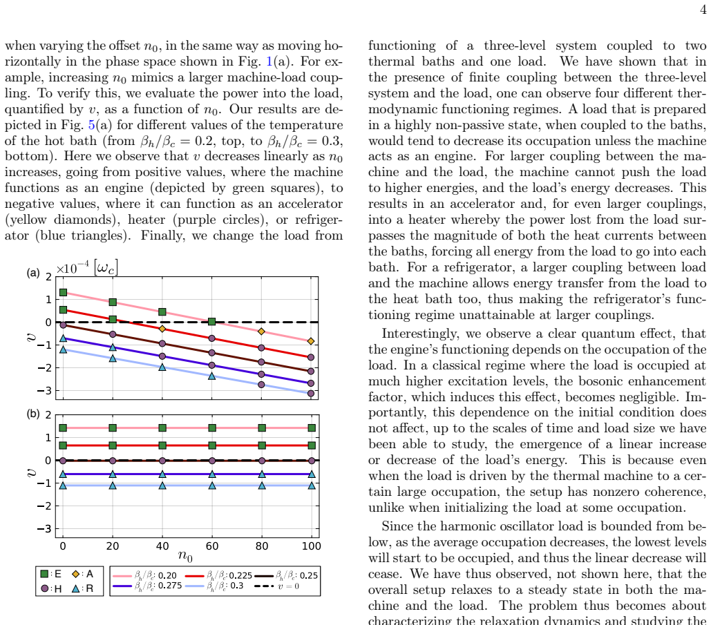
- For a bosonic load, the functioning regime depends on the initial occupation through the $\sqrt{n_0}$ enhancement, so preparing the load differently is equivalent to moving horizontally in the regime diagram.
- A local master-equation treatment, which neglects the counter-rotating machine-load coupling, does not show these regime changes, so global treatments are necessary already at moderate coupling.
- Since the drift velocity can change sign at resonance for large $g$, the resonant engine mechanism is replaced by higher-order processes, which should be observable as a sign change in the load's mean energy rate.
Reading between the lines
- If the regime diagram is robust, then measuring the load's drift velocity $v$ as a function of $g$ in a cavity or trapped-ion realization would provide a direct signature of the critical coupling $g/\hbar\omega_c \simeq 0.344$ where refrigeration vanishes.
- The bosonic-enhancement sensitivity suggests that the same device could function as a sensor of the load's excitation number: the steady-state heat currents carry information about the initial occupation of the load.
- The authors' caveat that the linear drift ceases when the load reaches low occupations implies that the long-time fate of the load is a non-equilibrium steady state, not indefinite biased diffusion; characterizing that steady state is a natural follow-up.
- If the secular approximation breaks for the harmonic oscillator's equally spaced spectrum, the quantitative thresholds such as $0.344$ may shift, so a Redfield-II or beyond-Markov calculation is the needed cross-check for the exact values.
Editorial analysis
A structured set of objections, weighed in public.
Referee Report
Summary. The manuscript studies an autonomous three-level thermal machine coupled to a harmonic-oscillator load and two thermal baths, modeled by a global GKSL master equation. It reports a two-parameter phase diagram in the machine-load coupling g and the inverse hot-bath temperature βh, identifying four functioning regimes (engine, accelerator, heater, refrigerator), with the refrigerator disappearing for g/ℏωc ≳ 0.344. It further shows that a bosonic enhancement factor makes the dynamics sensitive to the load's initial occupation, an effect absent for a ladder load.
Significance. If correct, the paper establishes the machine-load coupling as a control parameter for thermodynamic functioning and identifies a genuinely quantum (bosonic-enhancement) mechanism for regime switching. The paper's analytic anchors—the weak-coupling Scovil-Schulz boundary, the biased-diffusion description, and the g → g√n0 Taylor-equivalence check—are concrete and reproducible, and the numerical phase diagram is computed from a fixed Hamiltonian with no parameters fitted to the target regimes. The main unresolved point is the quantitative validity of the secular global master equation at the couplings where the new regimes appear; this is testable and should be settled before publication.
major comments (3)
- [Appendix A, Eq. (3), Fig. 1(a)] Appendix A states that the global GKSL master equation agrees quantitatively with the Redfield-II equation, but no comparison is displayed. Since the central regime diagram and the disappearance of the refrigerator at g/ℏωc ≳ 0.344 are computed with Eq. (3), this validation claim is load-bearing. Please include a quantitative comparison of v, Qh, and Qc (or of the full regime boundaries) between GME and Redfield-II for representative parameters across the transitions, including the large-coupling region, and state the maximal discrepancy.
- [Appendix A, Eq. (3), Fig. 2] The secular approximation in Eq. (3) requires dressed Bohr frequencies to be separated by more than the dissipative scale γ ∼ ηωc. For the resonant oscillator load (ωl = ωe), the dressed states formed from |2,n⟩ and |3,n−1⟩ have frequencies near ωc shifted by ±g√n, so the spacing between vertical machine transitions at neighbouring occupations n and n+1 is of order g/(2√n). Since the load occupation grows linearly in time during engine operation, this spacing eventually becomes much smaller than γ, so the secular approximation can fail precisely in the long-time dynamics used to assign regimes. The 40-times speed advantage of the GME is not a substitute for a convergence check; please show Redfield-II data at long times or a spectral-separation analysis.
- [Model and numerics (Eq. (3), Figs. 1–5)] The manuscript never specifies the oscillator Hilbert-space truncation dimension or the convergence tests used to ensure that the biased diffusion and the regime boundaries are free of finite-size effects. This is essential for reproducibility, because the mean occupation changes linearly and the variance grows linearly in time; a too-small truncation would artificially reflect the wavepacket, and a too-large one would exacerbate the secular-approximation concern in Major Comment 2. Please state N_trunc and show convergence of v and the phase boundaries with N_trunc.
minor comments (5)
- [Appendix C, Eq. (C2)] In Eq. (C2), with r+ and r− defined as the rates for n→n+1 and n→n−1, the incoming terms are interchanged; as written, the drift coefficient in Eq. (C4) has the opposite sign from Eq. (C5). Please correct the notation or the signs.
- [Fig. 3(a) and main text] The caption and text use 'g/ℏω' instead of 'g/ℏωc'; please make the notation consistent.
- [Main text, Fig. 1] The four functioning regimes are defined only through the schematics in Fig. 1(b–e); please state the sign conditions on Pl, Qh, and Qc in the main text so the phase boundaries are unambiguous.
- [Main text, Fig. 5] The text says the offset n0 modifies the matrix elements √n → √n+n0, while Fig. 5(a) is described as 'initial offset n0'; please clarify whether n0 is an initial Fock-state occupation or a model parameter, and specify how finite-size effects were excluded.
- [Eq. (7), Appendix C] The ergotropy rate in Eq. (7) is singular at t = 0 and the derivation assumes a broad Gaussian; this is acceptable for the long-time claim, but a brief statement of the regime of validity would help the reader.
Circularity Check
No circular derivation: the regime map is computed from a fixed model with no fitted parameters; the main caveats concern master-equation validity, not circularity.
full rationale
The paper's central claim—that finite machine-load coupling g produces engine, accelerator, heater, and refrigerator regimes (Fig. 1(a))—is obtained by numerically integrating the fixed model in Eq. (3) with stated parameters (η=0.005ωc, βc=2(ℏωc)^{-1}, ωl=ωe=3ωc) and no parameter fitted to the target regimes; the regimes are diagnosed by the signs of the computed currents ˙Q_h, ˙Q_c, and P_l, which is a classification, not an input. The weak-coupling engine/refrigerator boundary reproduces the independent Scovil-Schulz condition βhωh=βcωc (App. D), giving an external benchmark. The g→g√n0 relation is derived by Taylor expansion of √(n0+n) and independently cross-checked by comparing offset-ladder and increased-g simulations (footnote [33]), so it is not a fitted input called a prediction. Self-citations [18,19,25] are background, observational, or standard technical references and are not load-bearing for the new regime map. The flagged limitation is Appendix A's statement that 'We have compared the results from the GME with those from Redfield-II, and we have observed quantitative agreement' without showing the comparison; this is an unverified validity claim about the master equation at finite coupling and affects confidence in quantitative boundaries, but it is not a circular step because the GME is not constructed from the results it predicts. Score 2 reflects minor non-load-bearing self-citation and an unreported validation, not circularity.
Assumptions & free parameters
free parameters (5)
- g (machine-load coupling) =
0 to ~0.35 ℏωc
- η (bath spectral coupling) =
0.005 ωc
- βc and βh (inverse temperatures) =
βc = 2(ℏωc)^{-1}, βh/βc between 0.15 and 0.3 in the figures
- ωl and ωe (load and machine frequencies) =
ωl = ωe = 3 ωc
- n0 (initial occupation offset) =
varied up to large values (the text says 'large off-settings')
assumptions (3)
- domain assumption Global GKSL master equation with secular approximation (Eq. 3, App. A) correctly describes the machine+load dynamics
- domain assumption The load's occupation distribution follows a classical biased diffusion with Gaussian profile and stays away from n=0 (App. C)
- standard math Taylor expansion √(n+n0) ≈ √n0 for n0 >> n justifies the effective coupling g → g√n0
Cite this review
Pith. "Pith review of Emergence of thermodynamic functioning regimes from finite coupling between a quantum thermal machine and a load." pith.science (2026). https://pith.science/paper/A2Y5RI2Q
@misc{pith2026250601852,
  author       = {Pith},
  title        = {Pith review of: Emergence of thermodynamic functioning regimes from finite coupling between a quantum thermal machine and a load},
  year         = {2026},
  howpublished = {\url{https://pith.science/paper/A2Y5RI2Q}},
  note         = {Machine review of arXiv:2506.01852}
}
read the original abstract
Autonomous quantum thermal machines are particularly suited to understand how correlations between thermal baths, a load, and a thermal machine affect the overall thermodynamic functioning of the setup. Here, we show that by tuning the operating temperatures and the magnitude of the coupling between machine and load, the thermal machine can operate in four modes: engine, accelerator, heater, or refrigerator. In particular, we show that as we increase the coupling strength, the engine mode is suppressed, and the refrigerator mode is no longer attainable, leaving the heater as the most pronounced functioning modality, followed by the accelerator. This regime switching can be amplified by quantum effects, such as the bosonic enhancement factor for a harmonic oscillator load, which modifies the effective machine-load coupling, making the thermodynamic functioning sensitive to the initial preparation of the load.
Figures


Figures from the paper (2 more)

Reference graph
Works this paper leans on
-
[1]
Müller, A History of Thermodynamics: The Doctrine of Energy and Entropy (Springer, 2007)
I. Müller, A History of Thermodynamics: The Doctrine of Energy and Entropy (Springer, 2007)
work page 2007
-
[2]
A. Solfanelli, M. Falsetti, and M. Campisi, Phys. Rev. B 101, 054513 (2020)
work page 2020
-
[3]
R. S. Watson and K. V. Kheruntsyan, Quantum many- body thermal machines enabled by atom-atom correla- tions (2025), arXiv:2308.05266 [cond-mat.quant-gas]
arXiv 2025
-
[4]
Leveraging quantum statistics to enhance heat engines
K. Menon, T. Busch, and T. Fogarty, Leveraging quantum statistics to enhance heat engines (2025), arXiv:2503.19341 [quant-ph]
work page Pith review arXiv 2025
-
[5]
A. Solfanelli, G. Giachetti, M. Campisi, S. Ruffo, and N. Defenu, New Journal of Physics25, 033030 (2023)
work page 2023
-
[6]
Binder, Thermodynamics in the Quantum Regime: Fundamental Aspects and New Directions , edited by L
F. Binder, Thermodynamics in the Quantum Regime: Fundamental Aspects and New Directions , edited by L. A. Correa, C. Gogolin, J. Anders, and G. Adesso, Fun- damental Theories of Physics, Vol. 195 (Springer Inter- national Publishing)
-
[7]
Kosloff, Entropy15, 2100 (2013)
R. Kosloff, Entropy15, 2100 (2013)
2013
-
[8]
S. Deffner and S. Campbell,Quantum Thermodynamics, 2053-2571 (Morgan and Claypool Publishers, 2019)
work page 2019
Show all 47 references
-
[9]
Vinjanampathy and J
S. Vinjanampathy and J. Anders, Contemporary Physics 57, 545 (2016)
2016
-
[10]
Campbell, I
S. Campbell, I. D’Amico, M. A. Ciampini, J. Anders, N. Ares, et al., Roadmap on quantum thermodynamics (2025), arXiv:2504.20145 [quant-ph]
2025
-
[11]
N. M. Myers, O. Abah, and S. Deffner, AVS Quantum Science 4, 027101 (2022)
2022
-
[12]
L. M. Cangemi, C. Bhadra, and A. Levy, Physics Reports 1087, 1 (2024)
2024
-
[13]
J. V. Koski, V. F. Maisi, J. P. Pekola, and D. V. Averin, Proceedings of the National Academy of Sciences111, 13786 (2014)
2014
-
[14]
Klatzow, J
J. Klatzow, J. N. Becker, P. M. Ledingham, C. Wein- zetl, K. T. Kaczmarek, D. J. Saunders, J. Nunn, I. A. Walmsley, R. Uzdin, and E. Poem, Phys. Rev. Lett.122, 110601 (2019)
2019
-
[15]
Maslennikov, S
G. Maslennikov, S. Ding, R. Hablützel, J. Gan, A. Roulet, S. Nimmrichter, J. Dai, V. Scarani, and D. Matsukevich, Nature Communications10, 202 (2019)
2019
-
[16]
von Lindenfels, O
D. von Lindenfels, O. Gräb, C. T. Schmiegelow, V. Kaushal, J. Schulz, M. T. Mitchison, J. Goold, F. Schmidt-Kaler, and U. G. Poschinger, Phys. Rev. Lett. 123, 080602 (2019)
2019
-
[17]
J. P. S. Peterson, T. B. Batalhão, M. Herrera, A. M. Souza, R. S. Sarthour, I. S. Oliveira, and R. M. Serra, Phys. Rev. Lett.123, 240601 (2019)
2019
-
[18]
Van Horne, D
N. Van Horne, D. Yum, T. Dutta, Z. Gong, D. Poletti, P. Hänggi, J. Gong, and D. Poletti, npj Quantum Inform- ation 6, 37 (2020)
2020
-
[19]
C. Teo, U. Bissbort, and D. Poletti, Phys. Rev. E95, 030102 (2017)
2017
-
[20]
Roulet, S
A. Roulet, S. Nimmrichter, J. M. Arrazola, S. Seah, and V. Scarani, Phys. Rev. E95, 062131 (2017)
2017
-
[21]
S. Seah, S. Nimmrichter, and V. Scarani, New Journal of Physics 20, 043045 (2018)
2018
-
[22]
Gorini, A
V. Gorini, A. Kossakowski, and E. C. G. Sudarshan, Journal of Mathematical Physics17, 821 (1976)
1976
-
[23]
Lindblad, Communications in Mathematical Physics 48, 119 (1976)
G. Lindblad, Communications in Mathematical Physics 48, 119 (1976)
1976
-
[24]
H. P. Breuer and F. Petruccione, The theory of open quantum systems (Oxford University Press, Great Clar- endon Street, 2002)
2002
-
[25]
G. T. Landi, D. Poletti, and G. Schaller, Reviews of Mod- ern Physics94, 045006 (2022)
2022
-
[26]
Lett.67, 565 (2004)
A.E.Allahverdyan, R.Balian,andT.M.Nieuwenhuizen, Europhys. Lett.67, 565 (2004)
2004
-
[27]
Goold, and F
G.Francica, F.C.Binder, G.Guarnieri, M.T.Mitchison, J. Goold, and F. Plastina, Phys. Rev. Lett.125, 180603 (2020)
2020
-
[28]
2, 262 (1959)
H.E.D.ScovilandE.O.Schulz-DuBois,Phys.Rev.Lett. 2, 262 (1959)
1959
-
[29]
Geva and R
E. Geva and R. Kosloff, Phys. Rev. E49, 3903 (1994)
1994
-
[30]
Geva and R
E. Geva and R. Kosloff, The Journal of Chemical Physics 104, 7681 (1996)
1996
-
[31]
Geva, Journal of Modern Optics49, 635 (2002)
E. Geva, Journal of Modern Optics49, 635 (2002)
2002
-
[32]
Singh, Phys
V. Singh, Phys. Rev. Res.2, 043187 (2020)
2020
-
[33]
We also verified this by comparing two equivalent cases: (i) offsetting the ladder byn0 while keeping g fixed, and (ii) increasing g to c0g√n0 without offset
This relation can be analytically derived by the Taylor expansion of √n0 + n under the approximationn0 ≫ n. We also verified this by comparing two equivalent cases: (i) offsetting the ladder byn0 while keeping g fixed, and (ii) increasing g to c0g√n0 without offset
-
[34]
Scovil, Journal of Applied Physics30, 1113 (1959)
J.E.Geusic, E.O.S.Bois, R.W.DeGrasse,andH.E.D. Scovil, Journal of Applied Physics30, 1113 (1959)
1959
-
[35]
M. A. Sillanpää, J. Li, K. Cicak, F. Altomare, J. I. Park, R. W. Simmonds, G. S. Paraoanu, and P. J. Hakonen, Phys. Rev. Lett.103, 193601 (2009)
2009
-
[36]
K. S. Kumar, A. Vepsäläinen, S. Danilin, and G. S. Paraoanu, Nature Communications7, 10628 (2016)
2016
-
[37]
H. K. Xu, C. Song, W. Y. Liu, G. M. Xue, F. F. Su, H. Deng, Y. Tian, D. N. Zheng, S. Han, Y. P. Zhong, H. Wang, Y. xi Liu, and S. P. Zhao, Nature Communic- ations 7, 11018 (2016)
2016
-
[38]
Vepsäläinen, S
A. Vepsäläinen, S. Danilin, and G. S. Paraoanu, Science Advances5, eaau5999 (2019)
2019
-
[39]
Blatt and C
R. Blatt and C. Roos, Nature Physics8, 277 (2012)
2012
-
[40]
Barzanjeh, A
S. Barzanjeh, A. Xuereb, S. Gröblacher, M. Paternostro, C. A. Regal, and E. M. Weig, Nature Physics 18, 15 (2022). 6
2022
-
[41]
Krämer, D
S. Krämer, D. Plankensteiner, L. Ostermann, and H. Ritsch, Computer Physics Communications227, 109 (2018)
2018
-
[42]
https://www.nscc.sg/
-
[43]
Tupkary, A
D. Tupkary, A. Dhar, M. Kulkarni, and A. Purkayastha, Phys. Rev. A105, 032208 (2022)
2022
-
[44]
De Chiara, G
G. De Chiara, G. Landi, A. Hewgill, B. Reid, A. Ferraro, A. J. Roncaglia, and M. Antezza, New Journal of Physics 20, 113024 (2018)
2018
-
[45]
Levy and R
A. Levy and R. Kosloff, Europhysics Letters107, 20004 (2014). Appendix A: Derivation of the Global Master Equation We outline the derivation of the Redfield and GKSL- type master equations used to describe the dynamics of a quantum system weakly coupled to thermal reservoirs. ...
2014
-
[46]
To find the equation of motion for this distribution, we consider a specific level n at time t, and consider all the processes that cause it to change
Partial differential equation for classical biased diffusion We define a probability distributionp(n, t) that tells us the probability of being in thenth energy level of an oscillator that changes with timet. To find the equation of motion for this distribution, we consider a ...
-
[47]
(C5), assuming an initial probability distribution loc- alized at leveln0 at time t = 0, is given by p(n, t) = 1√ 4πDt exp − (n − vt − n0)2 4Dt
Analytical Expressions for Energy, Entropy, and Ergotropy from Classical Biased Diffusion The solution to the biased diffusion equation in Eq. (C5), assuming an initial probability distribution loc- alized at leveln0 at time t = 0, is given by p(n, t) = 1√ 4πDt exp − (n − vt −...
Reviewed August 7, 2026 · model on record in the stance chip above.
Discussion (0). Sign in to comment.