REVIEW 3 major objections 5 minor 62 references
Sensitivity-Aware Density Estimation in Multiple Dimensions
T0 review · 3 major / 5 minor · reviewed 2026-08-07 · deepseek-v4-flash
Pith's one-line read This paper proposes a density estimator that folds detector sensitivity into the normalization as a measure and claims it outperforms kernel and histogram baselines in multidimensional density estimation and PET rebinning.
desk verdict Sensitivity-as-measure density estimation on spline grids is a genuine contribution, but the strict-concavity proof has a flat-direction gap and the experiments lack error bars. read the letter →
The pith
A machine-rendered reading of the paper's core claim, the machinery that carries it, and where it could break.
The reading
What carries the argument
The load-bearing object is the exponential-family cardinal B-spline density $\hat\pi(x;c)=\exp(\sum_{m\in M} c[m]\varphi_m(x))$, where $\varphi$ is a separable tensor product of one-dimensional B-splines on a uniform grid. It does two jobs at once: the exponential keeps the density nonnegative, and the uniform grid turns normalization, density evaluation, and Hessian computation into separable convolutions. The sensitivity map $\xi$ is attached as a Lebesgue-Stieltjes measure in the normalization $E(\cdot)=\int_X \cdot\,\xi\,dx$, which is what avoids the unstable pointwise inversion. The regularizer is the nuclear norm of the Hessian of the log-density, $R(c)=\int_X \|H\{\log\hat\pi\}\|_{S_1}$, approximated on the grid by an $\ell^1$ sum of Schatten norms; it promotes low-rank Hessians, i.e., locally affine log-densities. Optimization is an accelerated proximal-gradient scheme with an adaptive Lipschitz bound and a dual-based proximal operator for the Hessian-Schatten norm.
What would settle it
The decisive test is to take a known target density and a sensitivity map that is exactly zero on a region of positive measure, generate samples by thinning, and evaluate the mean-squared error of the regularized spline estimate against the target: the paper's guarantee relies on $\xi>0$ almost everywhere, so the estimate should degrade or fail exactly in that setup.
Extended reading notes
Core claim
The discovery is a parameterization and regularization recipe that makes sensitivity-aware density estimation stable in multiple dimensions. Where weighted kernel density estimation sets each sample's weight to the inverse detection probability, this method folds $\xi$ into the expectation operator $\mathbb{E}(\cdot)=\int_X \cdot\,\xi(x)\,dx$, so the log-likelihood's normalization term automatically balances data in low- and high-sensitivity zones. The density is parameterized as $\hat\pi(x;c)=\exp(\sum_{m\in M} c[m]\varphi_m(x))$ with separable cardinal B-splines, so all integrals, derivatives, and evaluations reduce to convolutions on a grid with chosen boundary conditions. Adding $\lambda \int_X \|H\log\hat\pi\|_{S_1}$ as a regularizer promotes splines whose log-density is locally affine, which acts as automatic knot selection and gives robustness to the choice of $\lambda$. Experiments on standard 2D and 3D densities and on PET sinograms are reported to show lower mean-squared error than kernel and histogram estimators across $10^2$ to $10^6$ samples, and to show that resampled sinograms improve PET reconstructions.
Load-bearing premise
The method assumes the sensitivity map $\xi$ is known, positive almost everywhere, and statistically independent of the phenomenon being measured, so the observed density is exactly $\pi\xi/\int_X \pi\xi$; if that assumption fails, the estimate converges to the wrong density.
Editorial extensions
If this is right
- Because $\xi$ is integrated rather than divided, estimates remain stable in regions where detection probability is small, as long as the normalization integrals are well defined.
- Grid-based computation decouples cost from sample count: optimization and evaluation time stay roughly flat from $10^2$ to $10^6$ samples in the reported 2D tests, which matters for PET data that routinely exceed $10^6$ samples.
- The nuclear-norm regularizer acts as a bandwidth selector: it automatically deactivates knots in 1D and favors planar log-density regions in higher dimensions, so results are comparatively insensitive to grid size and to the regularization parameter $\lambda$.
- On standard densities UGL and GG in 2D and 3D, the method is reported to dominate histogram and kernel estimators in mean-squared error across the whole tested sample range, with the largest margin in 3D.
- In PET, sinograms resampled with this estimator produce sharper reconstructions and better contrast than histogram or kernel rebinning, including on a real amyloid scan dataset.
Reading between the lines
- If the sensitivity map is misspecified or detection is not independent of the phenomenon, the normalization-based estimator targets $\pi\xi/\int\pi\xi$ rather than the true density; a natural extension would be to place a prior on $\xi$ or estimate it jointly, but the paper does not address this.
- The exponential-family form gives the estimate a built-in normalization and strict concavity of the log-likelihood, so plug-in confidence bands from observed Fisher information are a plausible extension, though the paper stops at point estimates.
- Because runtime depends on the grid rather than on the number of samples, the method is a candidate for streaming or online density estimation where kernel evaluation costs would grow without bound; that application is not tested here.
- The same measure-based weighting could carry over to Bayesian or variational density estimation, or to other inverse problems beyond PET, wherever a known spatially varying detection probability is available.
Editorial analysis
A structured set of objections, weighed in public.
Referee Report
Summary. The paper introduces regularized density splines (RDS), a multidimensional density estimator for samples acquired with spatially varying detection probability. The unknown density is parameterized as the exponential of a tensor-product B-spline series on a uniform grid; the known sensitivity map enters as the reference measure in the likelihood normalization rather than through pointwise inversion of the weights. The negative log-likelihood is augmented with a Hessian nuclear-norm penalty, and the resulting nonsmooth convex problem is solved by an accelerated proximal-gradient algorithm with an adaptive Lipschitz step. The method is evaluated against kernel and histogram estimators on synthetic distributions and on PET sinogram rebinning/reconstruction tasks.
Significance. RDS addresses a practically important problem: stable weighted density estimation with heterogeneous sensitivity and general boundary conditions. The measure-based normalization is a principled alternative to the unstable inversion used in weighted KDE. The paper is unusually complete on the implementation side: evaluation and derivative computations are convolution-based, the proximal operator is derived, software is released, and tests include realistic PET phantoms. If the identified proof issues are corrected, the method is a credible, computationally attractive alternative to KDE/HE in imaging applications.
major comments (3)
- [Section 3.3 and Section 4] The strict-concavity claim is false for the periodic B-spline bases used throughout the experiments. These bases satisfy sum_{m in M} phi_m(x) = 1 on the periodic domain. For tilde_c = alpha * 1, the inner term in Eq. (15) is constant, so the quadratic form is zero; hence the Hessian has a null direction, L_N(c + alpha*1) = L_N(c), and the regularizer R in Eq. (18) is invariant to constant shifts. J in Eq. (17) therefore has no unique minimizer, and the statement that J inherits strict convexity in Section 4 is incorrect. The normalized density estimate is still well defined, but an identifiability constraint, such as fixing one coefficient or the sum of coefficients, is required.
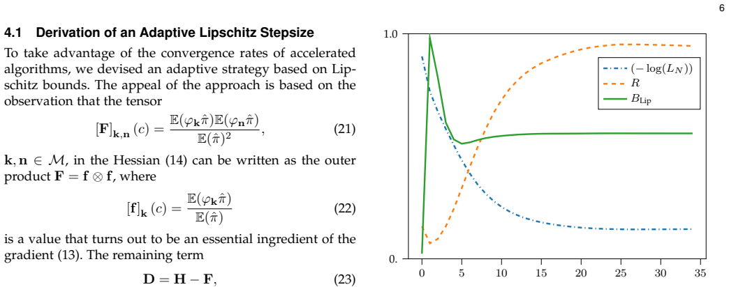
- [Section 4.1] The decomposition on which the adaptive step size rests is algebraically inconsistent with Eq. (14). Writing A_{kn} = E(phi_k phi_n pi), Eq. (14) yields H = -(N/E(pi)) A + N (f tensor f), where f is defined in Eq. (22). With F = f tensor f from Eq. (21), the remaining term D = H - F is -(N/E(pi)) A + (N-1) f tensor f, which is dense (a rank-one outer product is added to the banded matrix A) and is not guaranteed positive-definite. The 'banded' matrix used in the Gershgorin bound (26) is therefore not D, and B_Lip in Eq. (28) also appears to miss the factor N multiplying the outer-product term in Eq. (14). Since Algorithm 1 uses 1/B_Lip as the step size, the convergence justification in Section 4 is not yet established.
- [Section 5.3] The MSE comparisons appear to be based on a single sample realization per value of N. For small N, down to 10^2, the sampling variability of MSE is large, so the claim that RDS outperformed HE and KDE in all cases and over the whole range of samples is not established. The paper should provide repeated-trial means and dispersions, or confidence bands, and ideally a paired comparison across trials.
minor comments (5)
- [Abstract and Introduction] There is a typo 'This is is' in the first sentence of the Introduction, and 'BCS' should be written as 'BCs'.
- [Section 3.4] The approximation of the integral regularizer R in Eq. (18) by the discrete S_p-ell_1 sum in Eq. (20) is introduced without an error estimate; the manuscript should state whether the reported results use Eq. (18) or Eq. (20) and provide at least a heuristic justification of the discretization error.
- [Section 4.4] The display for the convergence criterion in Eq. (33) appears garbled, specifically the symbol sequence '1 <0'; the criterion should be rewritten as a standard control on the relative coefficient change.
- [Section 3.1] The consistency claim assumes that the sensitivity xi is known exactly and that detection is independent of the phenomenon, per Eq. (2), but no misspecification analysis is given; a brief robustness experiment with a perturbed xi would help the reader calibrate the PET claims.
- [Section 5.3.3 and Conclusion] There are minor typos: 'particulary' in Section 5.3.3 and 'futher' in the Conclusion should be corrected.
Circularity Check
Minor oracle-λ benchmarking in the Figure 7 'adapt' curve; the sensitivity-aware estimator itself is a self-contained MLE with external validation, so no significant circularity.
-
fitted input called prediction
[Section 5.3.1 (Quantitative Assessment) and Figure 7 caption]
"One where λ was adjusted at each number of samples according to the best MSE among five values (corresponding to five orders of magnitude). And another one where λ was fixed to the optimal value found for 10^2 samples. They both performed similarly (Figure 7). ... RDS (adapt) runs a small grid-search (three values) for the best λ at each number of samples, whereas (fixed) uses the same, fixed λ throughout all the range."
The adapt MSE-vs-samples curve is constructed by choosing λ at each N to minimize the same ground-truth MSE metric (Eq. (37)) that is then reported, so each plotted point is by construction the lower envelope of the λ-grid errors. The claim 'RDS outperformed HE and KDE in all cases and over the whole range of samples' uses this oracle-selected curve while KDE/HE receive only data-driven rule-of-thumb bandwidths (Scott, Freedman-Diaconis/Sturges), so part of the stated advantage is forced by the selection protocol rather than by the estimator. This is minor, not load-bearing, because the fixed-λ variant (λ set once at 10^2 samples) is reported to behave similarly, so the method's superiority does not reduce entirely to oracle tuning.
full rationale
The derivation chain is self-contained. The model ν = π̃ξ/∫π̃ξ (Eqs. (2)-(3)) is the density of detected events under the stated independence assumption; the exponential-family spline (5) with likelihood (11)-(12) is a true maximum-likelihood problem with direct derivatives (13)-(14); sensitivity enters only through the measure E(π̂)=∫π̂ξ (Eq. (4)), exactly the claimed avoidance of pointwise inversion, and no output quantity is defined in terms of another output quantity. The Hessian-Schatten regularizer (18)-(20) is an attributed published convex prior ([44], IEEE TIP 2013) whose stated assumptions do not include this paper's claims, so per the review protocol the self-citation does not raise the score; self-citation [50] only sources a synthetic PET ground truth, while validation also uses external benchmarks (Derenzo, Brain Phantom, Digimouse, real Amyloid data). Two flagged items do not change the verdict. (1) Correctness, not circularity: the strict-concavity claim ('The log-likelihood is therefore strictly concave', with Eq. (15) relying on 'the innermost term cannot be zero because the φ_m are linearly independent') is false for the periodic basis (38), which is a partition of unity: for c̃ ∝ 1 the quadratic form (15) vanishes exactly, the Hessian is singular, and both the log-likelihood and R(c) in (18) are invariant under adding a constant to the log-density, so the asserted unique optimum requires a gauge constraint; the normalized estimate is gauge-invariant, making this a fixable identifiability error rather than a collapse. (2) The one construction-level shortcut found is the Figure 7 'adapt' oracle-λ selection, recorded in steps above; it is mitigated by the reportedly similar 'fixed' curve. Also, the assumed-known sensitivity and independence are input assumptions, not derived outputs; the absence of misspecification analysis is a robustness gap, not circularity. Overall: no significant circularity, score 2.
Assumptions & free parameters
free parameters (3)
- Regularization parameter lambda =
user-chosen; grid-searched in experiments (e.g., 2^-4 to 2^4 in Figure 3, five values in Figure 7)
- Grid step mu (grid size M) =
per experiment; e.g., grids (44k, 44k) for k=1,2,3 in Figure 3
- Spline degree n =
n=1, chosen in Section 5.2.2
assumptions (6)
- domain assumption The sensitivity map xi is known, measurable, and positive almost everywhere on X.
- domain assumption The phenomenon and its detection are independent processes, so nu = pi * xi / integral(pi * xi).
- domain assumption The log-density of the target can be represented, or well approximated, by an exponential family of B-splines on a fixed uniform grid.
- domain assumption Boundary conditions of the domain are known and can be enforced through the spline basis and convolution operators.
- domain assumption The discrete Sp-l1 norm on the grid is a faithful proxy for the continuous Hessian-Schatten regularizer.
- standard math Convergence guarantees of accelerated proximal gradient with adaptive Lipschitz bounds and inexact prox apply.
Cite this review
Pith. "Pith review of Sensitivity-Aware Density Estimation in Multiple Dimensions." pith.science (2026). https://pith.science/paper/YPZ27MXH
@misc{pith2026250602323,
  author       = {Pith},
  title        = {Pith review of: Sensitivity-Aware Density Estimation in Multiple Dimensions},
  year         = {2026},
  howpublished = {\url{https://pith.science/paper/YPZ27MXH}},
  note         = {Machine review of arXiv:2506.02323}
}
read the original abstract
We formulate an optimization problem to estimate probability densities in the context of multidimensional problems that are sampled with uneven probability. It considers detector sensitivity as an heterogeneous density and takes advantage of the computational speed and flexible boundary conditions offered by splines on a grid. We choose to regularize the Hessian of the spline via the nuclear norm to promote sparsity. As a result, the method is spatially adaptive and stable against the choice of the regularization parameter, which plays the role of the bandwidth. We test our computational pipeline on standard densities and provide software. We also present a new approach to PET rebinning as an application of our framework.
Figures


Figures from the paper (13 more)


Reference graph
Works this paper leans on
-
[1]
A. Ihsani and T. H. Farncombe, “A Kernel Density Estimator- Based Maximum A Posteriori Image Reconstruction Method for Dynamic Emission Tomography Imaging,”IEEE Transactions on Image Processing, vol. 25, no. 5, pp. 2233–2248, May 2016
work page 2016
-
[2]
R. Y. Shopa, “Application of Kernel Density Estimation for Image Reconstruction in J-PET Scanners of High TOF Resolution,” in 2018 IEEE Nuclear Science Symposium and Medical Imaging Confer- ence Proceedings (NSS/MIC), Nov. 2018, pp. 1–3
work page 2018
-
[3]
Monolithic Picosecond Silicon Pixel Sensors for Future Physics: Experiments and Appli- cations,
G. Iacobucci, L. Paolozzi, and P . Valerio, “Monolithic Picosecond Silicon Pixel Sensors for Future Physics: Experiments and Appli- cations,”IEEE Instrumentation & Measurement Magazine, vol. 24, no. 9, pp. 5–11, Dec. 2021
work page 2021
-
[4]
Density Estimation for Positron Emission Tomography,
B. Pawlak and R. Gordon, “Density Estimation for Positron Emission Tomography,”Technology in Cancer Research & Treatment, vol. 4, no. 2, pp. 131–141, Apr. 2005. [Online]. Available: https://doi.org/10.1177/153303460500400202 14 Brain Phantom Ground Truth HE KDE RDS Brain Phantom Brain Phantom Digimouse Amyloid Fig. 15. Total-variation reconstructions afte...
-
[5]
I. M. Khater, I. R. Nabi, and G. Hamarneh, “A Review of Super-Resolution Single-Molecule Localization Microscopy Cluster Analysis and Quantification Methods,”Patterns, vol. 1, no. 3, p. 100038, Jun. 2020. [Online]. Available: https://www. sciencedirect.com/science/article/pii/S266638992030043X
work page 2020
-
[6]
Efficiency and time resolution of monolithic silicon pixel detectors in SiGe BiCMOS technology,
G. Iacobucci, L. Paolozzi, P . Valerio, T. Moretti, F. Cadoux, R. Cardarelli, R. Cardella, S. D ´ebieux, Y. Favre, D. Ferrere, S. Gonzalez-Sevilla, Y. Gurimskaya, R. Kotitsa, C. Magliocca, F. Martinelli, M. Milanesio, M. M ¨unker, M. Nessi, A. Picardi, J. Saidi, H. R ¨ucker, M. V . B. Pinto, and S. Zambito, “Efficiency and time resolution of monolithic si...
work page 2022
-
[7]
Weighted samples, kernel density estimators and convergence,
F. J. G. Gisbert, “Weighted samples, kernel density estimators and convergence,”Empirical Economics, vol. 28, no. 2, pp. 335–351, Apr
-
[8]
A practical implementation of weighted kernel density estimation for handling shape constraints,
M. A. Wolters and W. J. Braun, “A practical implementation of weighted kernel density estimation for handling shape constraints,”Stat, vol. 7, no. 1, p. e202, 2018. [Online]. Available: https://onlinelibrary.wiley.com/doi/abs/10.1002/sta4.202
Show all 62 references
-
[9]
Distinct formation history for deep-mantle domains reflected in geochemical differences,
L. S. Doucet, Z.-X. Li, H. Gamal El Dien, A. Pourteau, J. B. Murphy, W. J. Collins, N. Mattielli, H. K. H. Olierook, C. J. Spencer, and R. N. Mitchell, “Distinct formation history for deep-mantle domains reflected in geochemical differences,” Nature Geoscience, vol. 13, no. 7,...
2020
-
[10]
Improvements on Lightning Density Estimation Based on Analysis of Lightning Location System Performance Parameters: Brazilian Case,
V . Bourscheidt, O. Pinto, and K. P . Naccarato, “Improvements on Lightning Density Estimation Based on Analysis of Lightning Location System Performance Parameters: Brazilian Case,”IEEE Transactions on Geoscience and Remote Sensing, vol. 52, no. 3, pp. 1648–1657, Mar. 2014
2014
-
[11]
Short-Term Estimation and Prediction of Pedestrian Density in Urban Hot Spots Based on Mobile Phone Data,
J. Huo, X. Fu, Z. Liu, and Q. Zhang, “Short-Term Estimation and Prediction of Pedestrian Density in Urban Hot Spots Based on Mobile Phone Data,”IEEE Transactions on Intelligent Transportation Systems, vol. 23, no. 8, pp. 10 827–10 838, Aug. 2022
2022
-
[12]
An extended Weight Kernel Density Estimation model forecasts COVID-19 onset risk and identifies spatiotemporal variations of lockdown effects in China,
W. Shi, C. Tong, A. Zhang, B. Wang, Z. Shi, Y. Yao, and P . Jia, “An extended Weight Kernel Density Estimation model forecasts COVID-19 onset risk and identifies spatiotemporal variations of lockdown effects in China,”Communications Biology, vol. 4, no. 1, pp. 1–10, Jan. 2021....
2021
-
[13]
Recent Developments in Nonparametric Density Estimation,
A. J. Izenman, “Recent Developments in Nonparametric Density Estimation,”Journal of the American Statistical Association, vol. 86, no. 413, pp. 205–224, 1991. [Online]. Available: https://www.jstor.org/stable/2289732
1991
-
[14]
SciPy 1.0: fundamental algorithms for scientific computing in Python,
P . Virtanen, R. Gommers, T. E. Oliphant, M. Haberland, T. Reddy, D. Cournapeau, E. Burovski, P . Peterson, W. Weckesser, J. Bright, S. J. van der Walt, M. Brett, J. Wilson, K. J. Millman, N. Mayorov, A. R. J. Nelson, E. Jones, R. Kern, E. Larson, C. J. Carey, I. Polat, Y. Fen...
2020
-
[15]
Fast Kernel Density Estimation Using Gaussian Filter Approxi- mation,
M. Bullmann, T. Fetzer, F. Ebner, F. Deinzer, and M. Grzegorzek, “Fast Kernel Density Estimation Using Gaussian Filter Approxi- mation,” in2018 21st International Conference on Information Fusion (FUSION), Jul. 2018, pp. 1233–1240
2018
-
[16]
A fast and objective multidimensional kernel density estimation method: fastKDE,
T. A. O’Brien, K. Kashinath, N. R. Cavanaugh, W. D. Collins, and J. P . O’Brien, “A fast and objective multidimensional kernel density estimation method: fastKDE,”Computational Statistics & Data Analysis, vol. 101, pp. 148–160, Sep. 2016. [Online]. Available: https://www.scien...
2016
-
[17]
Efficient kernel den- sity estimation using the fast gauss transform with applications to color modeling and tracking,
A. Elgammal, R. Duraiswami, and L. Davis, “Efficient kernel den- sity estimation using the fast gauss transform with applications to color modeling and tracking,”IEEE Transactions on Pattern Analysis and Machine Intelligence, vol. 25, no. 11, pp. 1499–1504, Nov. 2003
2003
-
[18]
Nonparametric Density Estimation: Toward Computational Tractability,
A. G. Gray and A. W. Moore, “Nonparametric Density Estimation: Toward Computational Tractability,” inProceedings of the 2003 SIAM International Conference on Data Mining, May 2003, pp. 203–
2003
-
[19]
Kernel Density Estimation Using the Fast Fourier Transform,
B. W. Silverman, “Kernel Density Estimation Using the Fast Fourier Transform,”Journal of the Royal Statistical Society: Series C (Applied Statistics), vol. 31, no. 1, pp. 93–99, 1982. [Online]. Available: https://onlinelibrary.wiley.com/doi/abs/10. 2307/2347084
1982
-
[20]
Probit Transformation for Kernel Density Estimation on the Unit Interval,
G. Geenens, “Probit Transformation for Kernel Density Estimation on the Unit Interval,”Journal of the American Statistical Association, vol. 109, no. 505, pp. 346–358, Jan. 2014. [Online]. Available: https://doi.org/10.1080/01621459.2013.842173
2014
-
[21]
Bandwidth selection for kernel density estimation of fat-tailed and skewed distributions,
D. J. Henderson, A. Papadopoulos, and C. F. Parmeter, “Bandwidth selection for kernel density estimation of fat-tailed and skewed distributions,”Journal of Statistical Computation and Simulation, vol. 93, no. 12, pp. 2110–2135, Aug. 2023. [Online]. Available: https://doi.org/1...
2023
-
[22]
On Bandwidth Choice for Spatial Data Density Estimation,
Z. Jiang, N. Ling, Z. Lu, D. Tj ¨ostheim, and Q. Zhang, “On Bandwidth Choice for Spatial Data Density Estimation,”Journal of the Royal Statistical Society Series B: Statistical Methodology, vol. 82, no. 3, pp. 817–840, Jul. 2020. [Online]. Available: https://doi.org/10.1111/rssb.12367
2020 doi
-
[23]
Bandwidth Selection of Kernel Density Estimation for GIS-based Crime Occurrence Map Visualization,
Y. Kim, G. Kim, Y. Lee, and K. Jang, “Bandwidth Selection of Kernel Density Estimation for GIS-based Crime Occurrence Map Visualization,” in2020 International Conference on Information and Communication Technology Convergence (ICTC), Oct. 2020, pp. 1705–
2020
-
[24]
Kernel density estimation for circular data: a Fourier series-based plug-in approach for bandwidth selection,
C. Tenreiro, “Kernel density estimation for circular data: a Fourier series-based plug-in approach for bandwidth selection,”Journal of Nonparametric Statistics, vol. 34, no. 2, pp. 377–406, Apr
-
[25]
Bandwidth selection for kernel density estimation: a review of fully automatic selectors,
N.-B. Heidenreich, A. Schindler, and S. Sperlich, “Bandwidth selection for kernel density estimation: a review of fully automatic selectors,”AStA Advances in Statistical Analysis, vol. 97, no. 4, pp. 403–433, Oct. 2013. [Online]. Available: https://doi.org/10.1007/s10182-013-0216-y
2013 doi
-
[26]
Variable Kernel Density Estimation,
G. R. Terrell and D. W. Scott, “Variable Kernel Density Estimation,”The Annals of Statistics, vol. 20, no. 3, pp. 1236–1265, 1992, publisher: Institute of Mathematical Statistics. [Online]. Available: https://www.jstor.org/stable/2242011
1992
-
[27]
Estimation of Probability Density by an Orthogonal Series,
S. C. Schwartz, “Estimation of Probability Density by an Orthogonal Series,”Annals of Mathematical Statistics, vol. 38, no. 4, pp. 1261–1265, Aug
-
[28]
Approximation of Density Functions by Sequences of Exponential Families,
A. R. Barron and C.-H. Sheu, “Approximation of Density Functions by Sequences of Exponential Families,”The Annals of Statistics, vol. 19, no. 3, pp. 1347–1369, 1991. [Online]. Available: https://www.jstor.org/stable/2241953
1991
-
[29]
A study of logspline density estimation,
C. Kooperberg and C. J. Stone, “A study of logspline density estimation,”Computational Statistics & Data Analysis, vol. 12, no. 3, pp. 327–347, Nov. 1991. [Online]. Available: https: //www.sciencedirect.com/science/article/pii/016794739190115I
1991
-
[30]
Large-Sample Inference for Log-Spline Models,
C. J. Stone, “Large-Sample Inference for Log-Spline Models,”The Annals of Statistics, vol. 18, no. 2, pp. 717–741, 1990. [Online]. Available: https://www.jstor.org/stable/2242130
1990
-
[31]
Comparison of Parametric and Bootstrap Approaches to Obtaining Confidence Intervals for Logspline Density Estimation,
C. Kooperberg and C. J. Stone, “Comparison of Parametric and Bootstrap Approaches to Obtaining Confidence Intervals for Logspline Density Estimation,”Journal of Computational and Graphical Statistics, vol. 13, no. 1, pp. 106–122, 2004. [Online]. Available: https://www.jstor.or...
2004
-
[32]
Chapter 6: Density Estimation,
Y. K. N. Truong, C. Kooperberg, C. Stone, and M. Hansen, “Chapter 6: Density Estimation,” inStatistical Modeling with Spline Functions: Methodology and Theory. Springer Verlag New York, Sep. 2005
2005
-
[33]
Smoothing Spline Density Estimation: Theory,
C. Gu and C. Qiu, “Smoothing Spline Density Estimation: Theory,”The Annals of Statistics, vol. 21, no. 1, pp. 217–234, 1993. [Online]. Available: https://www.jstor.org/stable/3035588
1993
-
[34]
Bivariate Density Estimation with an Application to Survival Analysis,
C. Kooperberg, “Bivariate Density Estimation with an Application to Survival Analysis,”Journal of Computational and Graphical Statistics, vol. 7, no. 3, pp. 322–341, 1998. [Online]. Available: https://www.jstor.org/stable/1390707
1998
-
[35]
Fast B-spline transforms for continuous image representation and interpolation,
M. Unser, A. Aldroubi, and M. Eden, “Fast B-spline transforms for continuous image representation and interpolation,”IEEE Transactions on Pattern Analysis and Machine Intelligence, vol. 13, no. 3, pp. 277–285, Mar. 1991
1991
-
[36]
Contribution to the Problem of Approximation of Equidistant Data by Analytic Functions,
Schoenberg, I. J., “Contribution to the Problem of Approximation of Equidistant Data by Analytic Functions,”Quarterly of Applied Mathematics, vol. 4, no. 1, pp. 45–99, 1946
1946
-
[37]
Splines: a perfect fit for signal and image processing,
M. Unser, “Splines: a perfect fit for signal and image processing,” IEEE Signal Processing Magazine, vol. 16, no. 6, pp. 22–38, Nov. 1999
1999
-
[38]
Density estimation by total variation regularization,
R. Koenker and I. Mizera, “Density estimation by total variation regularization,” inAdvances in Statistical Modeling and Inference, ser. Series in Biostatistics, Mar. 2007, vol. 3, pp. 613–633
2007
-
[39]
A review of uncertainty quantification for density estimation,
S. McDonald and D. Campbell, “A review of uncertainty quantification for density estimation,”Statistics Surveys, vol. 15, pp. 1–71, Jan. 2021. [Online]. Available: https://projecteuclid. org/journals/statistics-surveys/volume-15/issue-none/ A-review-of-uncertainty-quantificati...
2021 doi
-
[40]
Improving “Fast Iterative Shrinkage-Thresholding Algorithm
J. Liang, T. Luo, and C.-B. Sch ¨onlieb, “Improving “Fast Iterative Shrinkage-Thresholding Algorithm”: Faster, Smarter, and Greedier,”SIAM Journal on Scientific Computing, vol. 44, no. 3, pp. A1069–A1091, Jun. 2022. [Online]. Available: https://epubs.siam.org/doi/10.1137/21M1395685
2022 doi
-
[41]
Proximal Newton-Type Methods for Minimizing Composite Functions,
J. D. Lee, Y. Sun, and M. A. Saunders, “Proximal Newton-Type Methods for Minimizing Composite Functions,”SIAM Journal on Optimization, vol. 24, no. 3, pp. 1420–1443, Jan. 2014. [Online]. Available: https://epubs.siam.org/doi/abs/10.1137/130921428
2014 doi
-
[42]
B-spline signal processing: Part I—Theory,
M. Unser, A. Aldroubi, and M. Eden, “B-spline signal processing: Part I—Theory,”IEEE Transactions on Signal Processing, vol. 41, no. 2, pp. 821–833, Feb. 1993
1993
-
[43]
A Fast Iterative Shrinkage-Thresholding Algorithm for Linear Inverse Problems,
A. Beck and M. Teboulle, “A Fast Iterative Shrinkage-Thresholding Algorithm for Linear Inverse Problems,”SIAM Journal on Imaging Sciences, vol. 2, no. 1, pp. 183–202, Jan. 2009. [Online]. Available: https://epubs.siam.org/doi/10.1137/080716542
2009 doi
-
[44]
Hessian Schatten- Norm Regularization for Linear Inverse Problems,
S. Lefkimmiatis, J. P . Ward, and M. Unser, “Hessian Schatten- Norm Regularization for Linear Inverse Problems,”IEEE Trans- actions on Image Processing, vol. 22, no. 5, pp. 1873–1888, May 2013
2013
-
[45]
Accelerated and Inexact Forward-Backward Algorithms,
S. Villa, S. Salzo, L. Baldassarre, and A. Verri, “Accelerated and Inexact Forward-Backward Algorithms,”SIAM Journal on Optimization, vol. 23, no. 3, pp. 1607–1633, Jan. 2013. [Online]. Available: https://epubs.siam.org/doi/10.1137/110844805
2013 doi
-
[46]
Adaptive Restart for Accelerated Gradient Schemes,
B. O’Donoghue and E. Cand `es, “Adaptive Restart for Accelerated Gradient Schemes,”Foundations of Computational Mathematics, vol. 15, no. 3, pp. 715–732, Jun. 2015. [Online]. Available: https://doi.org/10.1007/s10208-013-9150-3 16
2015 doi
-
[47]
Exact and approximate rebinning algorithms for 3- D PET data,
M. Defrise, P . Kinahan, D. Townsend, C. Michel, M. Sibomana, and D. Newport, “Exact and approximate rebinning algorithms for 3- D PET data,”IEEE Transactions on Medical Imaging, vol. 16, no. 2, pp. 145–158, Apr. 1997
1997
-
[48]
Development of ultrahigh resolution Si-PM-based PET system using 0.32mm pixel scintillators,
S. Yamamoto, H. Watabe, T. Watabe, H. Ikeda, Y. Kanai, Y. Ogata, K. Kato, and J. Hatazawa, “Development of ultrahigh resolution Si-PM-based PET system using 0.32mm pixel scintillators,” Nuclear Instruments and Methods in Physics Research Section A: Accelerators, Spectrometers,...
2016
-
[49]
The 100muPET project: A small-animal PET scanner for ultra-high resolution molecular imaging with monolithic silicon pixel detectors,
F. Cadoux, R. Cardella, G. Iacobucci, L. Iodice, D. Ferr `ere, S. Gonzalez-Sevilla, T. Kugathasan, F. Martinelli, L. Paolozzi, A. Picardi, J. Saidi, M. Vicente, and S. Zambito, “The 100muPET project: A small-animal PET scanner for ultra-high resolution molecular imaging with m...
2023
-
[50]
PET re- binning with regularized density splines,
A. Boquet-Pujadas, P . del Aguila Pla, and M. Unser, “PET re- binning with regularized density splines,” in2023 IEEE 20th International Symposium on Biomedical Imaging (ISBI), Apr. 2023, pp. 1–4
2023
-
[51]
Technical Note: Ultra high-resolution radiotracer-specific digital pet brain phantoms based on the BigBrain atlas,
M. A. Belzunce and A. J. Reader, “Technical Note: Ultra high-resolution radiotracer-specific digital pet brain phantoms based on the BigBrain atlas,”Medical Physics, vol. 47, no. 8, pp. 3356–3362, 2020. [Online]. Available: https://onlinelibrary.wiley. com/doi/abs/10.1002/mp.14218
2020 doi
-
[52]
Digimouse: a 3D whole body mouse atlas from CT and cryosection data,
B. Dogdas, D. Stout, A. F. Chatziioannou, and R. M. Leahy, “Digimouse: a 3D whole body mouse atlas from CT and cryosection data,”Physics in medicine and biology, vol. 52, no. 3, pp. 577–587, Feb. 2007. [Online]. Available: https://www.ncbi.nlm.nih.gov/pmc/articles/PMC3006167/
2007
-
[53]
Study protocol: Insight 46 – a neuroscience sub-study of the MRC National Survey of Health and Development,
C. A. Lane, T. D. Parker, D. M. Cash, K. Macpherson, E. Donnachie, H. Murray-Smith, A. Barnes, S. Barker, D. G. Beasley, J. Bras, D. Brown, N. Burgos, M. Byford, M. Jorge Cardoso, A. Carvalho, J. Collins, E. De Vita, J. C. Dickson, N. Epie, M. Espak, S. M. D. Henley, C. Hoskot...
2017
-
[54]
Single amyloid PET scan on the Siemens Biograph mMR,
P . J. Markiewicz, D. Cash, and J. M. Schott, “Single amyloid PET scan on the Siemens Biograph mMR,” Nov. 2018. [Online]. Available: https://zenodo.org/records/1472951
2018
-
[55]
Markoe,Analytic Tomography
A. Markoe,Analytic Tomography. Cambridge University Press, Jan. 2006
2006
-
[56]
Distributional Extension and Invertibility of the k-Plane Transform and Its Dual,
R. Parhi and M. Unser, “Distributional Extension and Invertibility of the k-Plane Transform and Its Dual,” Oct. 2023. [Online]. Available: http://arxiv.org/abs/2310.01233
2023 arXiv
-
[57]
Convex Quan- tization Preserves Logconcavity,
P . del Aguila Pla, A. Boquet-Pujadas, and J. Jald´en, “Convex Quan- tization Preserves Logconcavity,”IEEE Signal Processing Letters, vol. 29, pp. 2697–2701, 2022. Aleix Boquet-Pujadasreceived a bachelor’s degree in Mathematics and a bachelor’s de- gree in Physics from Univers...
1999
-
[211]
Available: https://epubs.siam.org/doi/10.1137/1
[Online]. Available: https://epubs.siam.org/doi/10.1137/1. 9781611972733.19
-
[1708]
Available: https://ieeexplore.ieee.org/abstract/ document/9289633?casa token=NPPsWi SeUAAAAA:2 fnEeBvsNoLgBIH-iI73vboMMzaWi-EwRhIcdQQgXTUSMab71m0CXLi5JjFAyGAArip4s59EA
[Online]. Available: https://ieeexplore.ieee.org/abstract/ document/9289633?casa token=NPPsWi SeUAAAAA:2 fnEeBvsNoLgBIH-iI73vboMMzaWi-EwRhIcdQQgXTUSMab71m0CXLi5JjFAyGAArip4s59EA
-
[1967]
Available: https://projecteuclid.org/ journals/annals-of-mathematical-statistics/volume-38/issue-4/ Estimation-of-Probability-Density-by-an-Orthogonal-Series/10
[Online]. Available: https://projecteuclid.org/ journals/annals-of-mathematical-statistics/volume-38/issue-4/ Estimation-of-Probability-Density-by-an-Orthogonal-Series/10. 1214/aoms/1177698795.full
-
[2003]
Available: https://doi.org/10.1007/s001810200134
[Online]. Available: https://doi.org/10.1007/s001810200134
-
[2022]
Available: https://doi.org/10.1080/10485252.2022
[Online]. Available: https://doi.org/10.1080/10485252.2022. 2057974
2022
Reviewed August 7, 2026 · model on record in the stance chip above.
Discussion (0). Sign in to comment.