REVIEW 2 major objections 4 minor 59 references
Ground states of classical spin polygons: Rigorous results and examples
T0 review · 2 major / 4 minor · reviewed 2026-08-07 · deepseek-v4-flash
Pith's one-line read Classical spin polygons—rings of unit spins with arbitrary nearest-neighbour couplings—have lowest-energy configurations that are only ever collinear or coplanar, and the paper proves the exact coupling at which a ring with one…
desk verdict Clean rigorous phase diagram for classical spin polygons; one real proof gap when the weakest FM bond is degenerate. read the letter →
The pith
A machine-rendered reading of the paper's core claim, the machinery that carries it, and where it could break.
The reading
What carries the argument
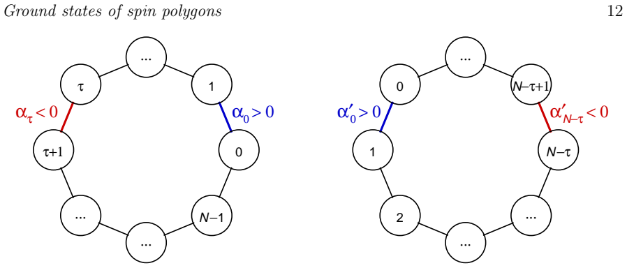
The central object is the difference-angle representation ψμ=φμ+1−φμ, whose sum obeys ψ0=2kπ−Σ_{μ=1}^{N-1}ψμ. The Lagrange parameter β:=α0 sinΨ=|αμ| sinψμ is constant across all bonds at any LEC, so all N−1 difference angles are functions of the single variable Ψ. After the spin-flip plus bond-inversion reduction, all nonzero ψμ lie in [0,π/2] in the regular domain, and the phase boundary is obtained from the fixed-point equation Ψ=f(Ψ) with f(Ψ)=Σ_{μ=1}^{N-1} arcsin((α0/|αμ|)sinΨ); the strict concavity of f forces the trivial collinear solution exactly when α0≤α(c).
What would settle it
Numerically minimize the energy of a hexagon whose two weakest ferromagnetic bonds have equal strength, sweeping α0 through α(c) and α(c′); if the observed collinear-to-coplanar boundaries or the energy at α0=|ατ| differ depending on which tie is labelled τ, then Theorem 3's classification is incomplete in the degenerate case.
Extended reading notes
Core claim
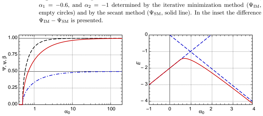
For a cycle of N classical spins with one antiferromagnetic bond α0>0 and all other bonds ferromagnetic, the lowest energy configuration is collinear if and only if α0≤α(c), where α(c)=(Σ_{μ=1}^{N-1}|αμ|^{-1})^{-1} is the harmonic mean of the ferromagnetic bond strengths and is strictly smaller than the weakest ferromagnetic bond |ατ|. For α(c)<α0<|ατ| the LEC is coplanar, unique, and varies analytically with α0, with a square-root onset of the summed difference angle Ψ at the transition. For α0 beyond |ατ|, a spin-flip transform maps the problem back to the regular domain and can produce a second transition to a collinear state; whether that transition occurs defines three types of α0-families that the paper classifies completely in terms of two further harmonic-like thresholds α(d) and α(d′).
Load-bearing premise
The phase diagram presumes a unique weakest ferromagnetic bond |ατ|; if several bonds tie for the minimum, the collinear state Ψ↑...↓ and the type classification in Theorem 3 depend on an arbitrary choice of τ, and the paper does not prove the phase boundaries are independent of that choice.
Editorial extensions
If this is right
- For any polygon with an odd number of antiferromagnetic bonds, the ground-state problem reduces to one antiferromagnetic bond, and the same two-parameter phase diagram applies regardless of ring size.
- The collinear-to-coplanar boundary is computable in closed form as a harmonic mean, so locating the transition in the regular domain requires no numerical minimization.
- In the coplanar phase all difference angles are determined by the single Lagrange parameter β, and the ground-state energy has exactly one maximum, at α0=α(em) where Ψ=π/2.
- For α0-families of type II, a second symmetry-related phase transition returns the LEC to the collinear state Ψ↑...↓, with a square-root law for Ψ approaching π.
- These exact classical results provide controlled starting points and selection rules for quantum spin-ring calculations at large spin.
Reading between the lines
- Extension (not in the paper): the same β-parameter fixed-point method should locate the collinear/coplanar boundary in open spin chains or ladders with one frustrated bond competing against a set of ferromagnetic bonds, with the harmonic mean replaced by the analogous inverse-sum over the chain.
- Extension (not in the paper): the degeneracy when several bonds share the minimal strength is an open robustness question; a perturbation that splits degenerate minimal bonds should produce phase boundaries that interpolate between the different τ choices, giving a measure of how stable the paper's type classification is.
- Extension (not in the paper): since β is the constant torque transmitted through the ring, the analytical formulas for β(α0) could be tested in mechanical hoop-and-spring models where the torque is directly measurable, not only in magnetic materials.
- Extension (not in the paper): the square-root onset of the coplanar order parameter at α(c) predicts a characteristic softening of a low-energy mode in quantum analogues at large spin, which could be probed by exact diagonalization or DMRG on small rings.
Editorial analysis
A structured set of objections, weighed in public.
Referee Report
Summary. The paper studies classical Heisenberg spin polygons with nearest-neighbor couplings αμ, i.e., energy E = Σ αμ sμ·sμ+1 on a cycle graph. It proves that every lowest-energy configuration (LEC) is either collinear or coplanar (Theorem 1), reduces arbitrary frustrated polygons by spin-flip and bond-inversion operations to the canonical case of one antiferromagnetic bond α0 > 0 and N−1 ferromagnetic bonds, and introduces difference angles ψμ together with a single Lagrange parameter β. In the regular domain 0 < α0 < |ατ|, where ατ is a weakest FM bond, the paper proves a sharp critical value α(c) (the harmonic mean of the |αμ|) separating the collinear phase from the coplanar phase (Theorem 2), and establishes uniqueness and analyticity of the coplanar solution (Proposition 4). A flip transformation transfers the results to the complementary domain |ατ| < α0 < ∞, yielding the second critical value α(c′) and the parameter value α(bm) at which β is maximal. This leads to a two-dimensional phase diagram in the (α0, |ατ|) plane and to a classification of one-parameter families into types II, Iβ, and Iα (Theorem 3). The paper closes with analytic and numerical examples for N = 3 and for a hexagon.
Significance. If the claims hold, this is a substantial and essentially complete analytic classification of classical spin-polygon ground states for arbitrary non-zero nearest-neighbor couplings. The main theorems are proved with elementary but careful calculus and concave-function arguments, and the critical values are parameter-free analytic expressions in the given bonds; the paper is self-contained and does not fit any quantity to the target result. The spin-flip reduction, the harmonic-mean transition point, and the square-root asymptotics at the transitions are concrete and potentially testable predictions for molecular-magnet rings. The main deficiency is the treatment of the case in which several FM bonds share the minimal strength; the proof route through the regular domain does not cover that case, and one displayed formula in the derivation of α(bm) is algebraically wrong, although the final formula appears to be correct.
major comments (2)
- [§5; Appendix B; Theorem 3] The complementary-domain phase diagram is not proved when the weakest FM bond is degenerate. The flip transformation (46a)–(46f) maps the complementary domain into the regular domain only if α′0 < |α′τ′|. If two distinct FM bonds satisfy |ατ| = |ασ|, then after the transformation one has α′0 = |ατ| and the bond corresponding to σ remains an FM bond of strength |ατ|, so α′0 = |α′τ′|. The transformed polygon therefore lies on the limit point treated in Appendix B, not in the open regular domain. Appendix B establishes only coplanarity at that point; it does not provide the bound ψ′μ ≤ π/2, the uniqueness of the fixed point, or the analyticity used in Proposition 4(iii) and Proposition 5. Hence Theorem 3(iv) and Proposition 5 are not rigorously established for degenerate minimal bonds, a case the paper explicitly includes in Proposition 2 and in the phase diagram (|ατ| = |ασ|). Since the paper claims to handle arbitrary couplings and to give precise phase boundaries, this gap is load-bearing. The statements may be true, but the proof needs either a separate treatment of the degenerate case or an explicit restriction excluding it from the theorems.
- [Eq. (48)] Equation (48) is algebraically inconsistent with the formula that follows it. Setting U = Σ_{μ=1}^{N−1} arcsin(|ατ|/|αμ|), Eq. (47) gives arcsin(|ατ|/α0) = π − U, hence α0 = |ατ| / sin U, not |ατ| / sin(U − π/2). Since U = π/2 + T with T = Σ_{μ≠τ} arcsin(|ατ|/|αμ|), the correct expression is |ατ| / cos T, which is exactly Eq. (49). The displayed denominator sin(U − π/2) would give |ατ| / sin T; for the N = 3 example of Sec. 7.1 this would yield α(bm) = 1 independently of |α1|, contradicting Eq. (73). Please correct or remove Eq. (48).
minor comments (4)
- [§4, Eqs. (38)–(40) and §5, Eqs. (56)–(58)] The square-root asymptotic expansions are asserted as following 'after some calculations' but no derivation is given. In a paper with 'rigorous results' in the title, please supply the Taylor-coefficient computation in an appendix or in a supplementary file.
- [§7, final paragraph] The sentence 'with the equations (??) and (66) given in proposition 5' contains a missing equation reference; it should refer to Eqs. (64) and (65).
- [Appendix A.3] In the last sentence of the proof of Theorem 2, 'the theorem 1' should be 'Theorem 2'.
- [Prop. 2 and §6] Because τ is arbitrary among equal-strength minimal bonds, it would help the reader to state explicitly that the quantities α(c), α(c′), α(d), and α(d′) are invariant under interchange of equal-strength bonds; this is true, but it is not said in the main text.
Circularity Check
Self-contained derivation; no circular reduction; minor non-circular proof gap at degenerate weakest-bond case.
full rationale
The paper's central claims are derived from the given couplings by explicit stationary-condition and convexity arguments, not by fitting or self-referential definitions. The critical values α(c), α(em), α(c'), α(bm), α(d), and α(d') are all explicit formulas in the input exchange integrals (Eqs. 33, 42, 49, 53, 54, 60), and the phase classification in Theorem 3 follows algebraically from these formulas. The spin-flip reduction in Section 5 is a standard energy-preserving transformation, and the regular-domain proof of Theorem 2 uses only the Hessian condition and the fixed-point equation f(Ψ)=Ψ (A.30); no target result is assumed. Citations to the authors' earlier works are contextual or concern numerical methods, and none is load-bearing for the mathematical results. The only caveat is a genuine proof gap, not circularity: Eq. (24) explicitly allows several bonds to attain the minimum |ατ|, and Appendix B shows the boundary case α0=|ατ| needs separate treatment. When the minimum is degenerate, the flip-transformed polygon lands on that boundary rather than in the open regular domain, so uniqueness and analyticity in the complementary domain are not proved there. This affects completeness and rigor, but it does not make any prediction equivalent to an input by construction. The derivation is therefore self-contained and non-circular.
Assumptions & free parameters
assumptions (4)
- domain assumption Each spin sµ is a unit vector in R3 and the energy is E = Σ αµ sµ·sµ+1 (periodic boundary conditions).
- standard math A lowest-energy configuration on the compact manifold (S2)^N is a local minimum and hence satisfies the stationary equation (3) and the Hessian condition (A.18).
- standard math The inverse function theorem and the matrix determinant lemma are valid for the smooth functions F and H constructed in the appendices.
- domain assumption The spin-flip operation combined with relabeling maps every configuration to an energy-equivalent configuration, so the regular-domain results transfer to the complementary domain.
Cite this review
Pith. "Pith review of Ground states of classical spin polygons: Rigorous results and examples." pith.science (2026). https://pith.science/paper/45BTMIOQ
@misc{pith2026250605838,
  author       = {Pith},
  title        = {Pith review of: Ground states of classical spin polygons: Rigorous results and examples},
  year         = {2026},
  howpublished = {\url{https://pith.science/paper/45BTMIOQ}},
  note         = {Machine review of arXiv:2506.05838}
}
read the original abstract
We present a comprehensive and rigorous analysis of the lowest energy configurations (LECs) of classical spin polygons characterized by arbitrary couplings between neighboring spin sites. Our study shows that these ground states exhibit either collinear or coplanar arrangements, which allows us to determine the precise boundaries between these two phases. By simultaneously applying a spin flip and a bond inversion, we simplify the LEC problem and reduce it to a specific scenario with predominantly ferromagnetic (FM) bonds and a single antiferromagnetic (AFM) bond. Hence, competing interactions are always present, but, nevertheless, in the well-defined ranges of the system parameters the collinear LEC is realized. The difference angles between neighboring spins within the LEC can be captured by a single Lagrange parameter. We analytically investigate its dependence on the AFM bond and arrive at revealing results. Similarly, we can analyze the energy of the LEC, which shows a pronounced maximum as a function of AFM bond. To illustrate our findings, we give various examples that clearly demonstrate these results.
Figures


Figures from the paper (5 more)



Reference graph
Works this paper leans on
-
[1]
Ground states of classical spin polygons: Rigorous results and examples
Introduction For years single molecule magnets have occupied a prominent place in c hemical and physical research, both experimental and theoretical. Recently , increasingly larger molecules containing, in addition to transition metals, also lanthanide io ns have been synthesized [1, 2, 3, 4, 5, 6, 7, 8]. In many cases, dimensions of the corresponding eig...
work page Pith review arXiv 2025
-
[2]
Classical spin polygons The systems considered in this work will be referred to as “polygons ”. In graph- theoretical terms [38] the system is assumed to be a cycle graph, i. e., a connected graph such that all vertices have exactly two neighbours. It is thus poss ible to label the N >2 vertices by the numbers µ = 0, 1,...,N − 1 such that the two neighbou...
-
[3]
[29, 41, 42, 43], see Figure 1
General properties of the LEC By flipping a sequence of spins sµ, µ = λ + 1,λ + 2,...,ν − 1,ν , and reversing the signs of the exchange integrals αλ and αν the energy of a polygon is left unchanged (cf. [29, 41, 42, 43], see Figure 1. By repeating this operation ever y even number of antiferromagnetic bonds can be transformed into ferromagnetic ones. Thus ...
-
[4]
Before we look at the theory behind this, a few preparatio ns are necessary
Regular domain: 0<α 0 < |ατ | In the regular domain there are two prominent values of α0: A critical point α(c) which marks a continuous phase transition between the collinear and the c oplanar ground state phase, and a point α(em) where the energy, written as a function of α0, assumes its maximum. Before we look at the theory behind this, a few preparati...
-
[5]
Complementary domain: |ατ |<α 0 < ∞ For α0 > |ατ | we cannot apply the theory presented in section 4. One way out is to flip the spins of number 1 ,...,τ and change the signs of the two coupling constants α0 andατ in order to obtain a polygon that lies in the regular domain and thus fulfi lls the conditions of the previous theory. It is advisable to renumbe...
-
[6]
Phase diagram We have seen in the previous section that there are three qualitativ e different possibilities for the one-parameter family of polygons/LECs which will be denote d by α0 ↦→ (P(α0), Ψ(α0)) and that these possibilities depend on the value of the weakest FM bond ατ . In this section we will investigate these dependencies more system atically and...
-
[7]
Phase diagram of an N = 6 polygon with FM bonds given by (75)
(60) Then the relationship between the type of the α0-family and the value of |ατ | is summarized in the following Theorem 3 If N >3 then: Ground states of spin polygons 15 Figure 3. Phase diagram of an N = 6 polygon with FM bonds given by (75). The coordinates are the AFM bond α0 and the weakest FM bond |ατ | = |α1|. The (red) solid curves separate the c...
-
[8]
However, we will start with a brief discussion of the methods for determining the required values
Examples In this section we present some results for different systems in ord er to illustrate the most important and the most characteristic features. However, we will start with a brief discussion of the methods for determining the required values. In g eneral, there are three types of problems. The easiest is to identify some values of th e parameter α0...
Show all 59 references
-
[9]
(70) For 0 < |ατ | < 1 a system is in the type II and the second phase transition takes place at α(c′) = |ατ | 1 − |ατ |. (71) The function β(α0) reaches its maximume when ψ1 =π/2, so from (19) we have α(bm) sin ( π/2 +ψ(bm) 2 ) =α(bm) cosψ(bm) 2 = |α1| = sinψ(bm) 2 , (72) hen...
-
[10]
A certain simplification is achieved by a repeated spin flip operation, which reduc es the problem to the special case α0 > 0, α1 < 0,...,α N −1 < 0
Summary The problem of finding all ground states of the N-spin polygon depends on an initially confusing set of N parameters, the exchange integrals α0,...,α N −1. A certain simplification is achieved by a repeated spin flip operation, which reduc es the problem to the special ca...
-
[11]
(A.12) We consider a modified spin configuration ~Ψ by setting ~ψλ = π 2 −δ and leaving the other angles unchanged. The energies of both configurations are given by E(Ψ) = α0 cos Ψ − N −1∑ µ=1, µ⁄=λ |αµ| cosψµ + |αλ| sinδ, (A.13) Ground states of spin polygons 24 E(~Ψ) = α0 cos (...
-
[12]
By proposition 2 we conclude ˆψµ =ˆΨ = N −1∑ ν=1 ˆψν = 0, (A.23) Ground states of spin polygons 25 for all 0 < µ < N
Only-if-part We assume that the LEC ˆΨ is collinear, i.e., sinˆΨ = sin ˆψµ = 0 (A.22) for all 0 <µ<N . By proposition 2 we conclude ˆψµ =ˆΨ = N −1∑ ν=1 ˆψν = 0, (A.23) Ground states of spin polygons 25 for all 0 < µ < N . It follows that the diagonal matrix A in (A.21) satisfie...
-
[13]
If-part We have to prove that any LEC is collinear for 0 < α0 ≤α(c). It is straightforward to show that the collinear state Ψ↑...↑ given by ψµ = 0 for all 0 <µ<N satisfies (17) and (A.18), and is hence a plausible candidate for an LEC (note that thes e conditions are only neces...
-
[14]
Baniodeh A, Magnani N, Lan Y, Buth G, Anson C E, Richter J, Affro nte M, Schnack J and Powell A K 2018 npj Quantum Materials 3 10
2018
-
[15]
47 3425–39
Majee M C, Towsif Abtab S M, Mondal D, Maity M, Weselski M, Witwick i M, Bie´ nko A, Antkowiak M, Kamieniarz G and Chaudhury M 2018 Dalton Trans. 47 3425–39
2018
-
[16]
Craig G A, Velmurugan G, Wilson C, Valiente R, Rajaraman G and Murr ie M 2019 Inorganic Chemistry 58 13815–25
2019
-
[17]
Fu Z, Qin L, Sun K, Hao L, Zheng Y Z, Lohstroh W, G¨ unther G, Rus sina M, Liu Y, Xiao Y, Jin W and Chen D 2020 npj Quantum Materials 5 32
2020
-
[18]
Antkowiak M, Majee M C, Maity M, Mondal D, Kaj M, Lesi´ ow M, Bie´ nko A, Kronik L, Chaudhury M and Kamieniarz G 2021 The Journal of Physical Chemistry C 125 11182–96
2021
-
[19]
Shukla P, Pal T K, Sahoo S C, Du M H, Kong X J and Das S 2021 ChemistrySelect 6 2456–63
2021
-
[20]
Tziotzi T G, Gracia D, Dalgarno S J, Schnack J, Evangelisti M, Bre chin E K and Milios C J 2023 Journal of the American Chemical Society 145 7743–7
2023
-
[21]
Jin P B, Luo Q C, Gransbury G K, Vitorica-Yrezabal I J, Hajdu T, S trashnov I, McInnes E J L, Winpenny R E P, Chilton N F, Mills D P and Zheng Y Z 2023 Journal of the American Chemical Society Published on-line 24 Nov. 2023
2023
-
[22]
Dmitriev D V, Krivnov V Y, Richter J and Schnack J 2019 Phys. Rev. B 99 094410
2019
-
[23]
Engelhardt L, Luban M and Schr¨ oder C 2006 Phys. Rev. B 74 054413
2006
-
[24]
Konstantinidis N P 2018 Journal of Magnetism and Magnetic Materials 449 55–62
2018
-
[25]
Schubert D, Richter J, Jin F, Michielsen K, De Raedt H and Steinige weg R 2021 Phys. Rev. B 104 054415
2021
-
[26]
Ueda H, Okunishi K, Krˇ cm´ ar R, Gendiar A, Yunoki S and NishinoT 2017 Phys. Rev. E 96 062112
2017
-
[27]
G´ omez Albarrac ´ ın F A and Pujol P 2018Phys. Rev. B 97 104419
-
[28]
Anisimov A V, Pini M G and Popov A P 2019 Journal of Magnetism and Magnetic Materials 479 105–13 Ground states of spin polygons 33
2019
-
[29]
Gemb´ e M, Schmidt H J, Hickey C, Richter J, Iqbal Y and Trebst S 2023 Phys. Rev. Res. 5 043204
2023
-
[30]
Furrer A and Waldmann O 2013 Rev. Mod. Phys. 85 367–420
2013
-
[31]
Timco G A, McInnes E J L and Winpenny R E P 2013 Chem. Soc. Rev. 42 1796–806
2013
-
[32]
Sharples J W, Collison D, McInnes E J L, Schnack J, Palacios E and E vangelisti M 2014 Nature Communications 5 5321
2014
-
[33]
McInnes E J L, Timco G A, Whitehead G F S and Winpenny R E P 2015 Angew. Chem. Int. Ed. 54 14244–69
2015
-
[34]
Ghirri A, Chiesa A, Carretta S, Troiani F, van Tol J, Hill S, Vitor ica-Yrezabal I, Timco G A, Winpenny R E P and Affronte M 2015 The Journal of Physical Chemistry Letters 6 5062–6
2015
-
[35]
Baker M L, Lancaster T, Chiesa A, Amoretti G, Baker P J, Bark er C, Blundell S J, Carretta S, Collison D, G¨ udel H U, Guidi T, McInnes E J L, M¨ oller J S, Mutka H, Ollivie r J, Pratt F L, Santini P, Tuna F, Tregenna-Piggott P L W, Vitorica-Yrezabal I J, Timco G A and Winpenn...
2016
-
[36]
Garlatti E, Bordignon S, Carretta S, Allodi G, Amoretti G, De R enzi R, Lascialfari A, Furukawa Y, Timco G A, Woolfson R, Winpenny R E P and Santini P 2016 Phys. Rev. B 93 024424
2016
-
[37]
Antkowiak M, Kamieniarz G, Timco G A, Tuna F and Winpenny R E P 201 9 Journal of Magnetism and Magnetic Materials 479 166–9
-
[38]
Schnack J 2019 Contemporary Physics 60 127–44
2019
-
[39]
Matysiak J and Lema´ nski R 2021 Phys. Rev. B 104 014431
2021
-
[40]
Pointillart F, Bernot K, Le Guennic B and Cador O 2023 Chem. Commun. 59 8520–8531
2023
-
[41]
Chiesa A, Santini P, Garlatti E, Luis F and Carretta S 2024 Reports on Progress in Physics 87 034501
2024
-
[42]
Toulouse 1977 Communcations de Physique 2 115–9
Toulouse G 1987 Theory of the frustration effect in spin glasses : I Spin Glass Theory and Beyond ed M´ ezard M, Parisi G and Virasoro M A (Singapore: World Scientific) pp 99–103 reprinted form: G. Toulouse 1977 Communcations de Physique 2 115–9
1987
-
[43]
Diep H T and Giacomini H 2004 Frustration—Exactly solved frustr ated models Frustrated Spin Systems ed Diep H T (Singapore: World Scientific) chap 1, pp 1–58
2004
-
[44]
Sriram Shastry B and Sutherland B 1981 Physica B+C 108 1069–70
1981
-
[45]
Voigt A, Richter J and Kr¨ uger S E 1995 Journal of Low Temperature Physics 99 381–3
1995
-
[46]
Richter J, Voigt A, Kr¨ uger S E and Gros C 1996 J. Phys. A: Math. Gen. 29 825–36
1996
-
[47]
Kamieniarz G, Florek W and Antkowiak M 2015 Phys. Rev. B 92 140411(R)
2015
-
[48]
Florek W, Antkowiak M and Kamieniarz G 2016 Phys. Rev. B 94 224421
2016
-
[49]
Florek W, Kamieniarz G and Marlewski A 2019 Phys. Rev. B 100 054434
2019
-
[50]
Naturforsch
Schmidt H J and Schr¨ oder C 2022 Z. Naturforsch. A 77 1099 – 1120
2022
-
[51]
Koh K M, Dong F, Ng K L and Tay E G 2015 Graph Theory (Singapore: World Scientific)
2015
-
[52]
Schmidt H J and Luban M 2003 J. Phys. A: Math. Gen. 36 6351–78
2003
-
[53]
Schmidt H J 2017 Theory of ground states for classical Heisenb erg spin systems I arXiv:1701.02489
2017 arXiv
-
[54]
Harary F 1953 The Michigan Mathematical Journal 2 143–146
1953
-
[55]
Mattis D C 2006 The Thory of Magnetism Made Simple (Singapore: World Scientific)
2006
-
[56]
Giampaolo S M, Gualdi G, Monras A and Illuminati F 2011 Phys. Rev. Lett. 107 260602
2011
-
[57]
Baez M L 2018 Numerical methods for frustrated magnetism Dissertation Freien Universit¨ at Berlin sec. 5.2.2
2018
-
[58]
Harville D A 1997 Matrix Algebra From a Statistician’s Perspective (New York, NY: Springer New York)
1997
-
[59]
Fritzsche K and Grauert H 2002 From Holomorphic Functions to Complex Manifolds (Graduate Texts in Mathematics vol 213) (New York, NY: Springer New York)
2002
Reviewed August 7, 2026 · model on record in the stance chip above.
Discussion (0). Sign in to comment.