REVIEW 3 major objections 5 minor 23 references
An Exploration of Vacuum-Decay Valleys
T0 review · 3 major / 5 minor · reviewed 2026-08-07 · deepseek-v4-flash
Pith's one-line read This paper argues that single-field false-vacuum decay can be organized as 2n+1 bounces—n bounce-antibounce pairs joined by pseudo-bounces—so standard overshoot/undershoot searches can miss half of the channels, sometimes the dominant one.
desk verdict The concrete examples and the antibounce concept are genuinely useful and should be taken seriously, but the advertised 2n+1 'general case' is an extrapolation from three potentials, not a proven theorem. read the letter →
The pith
A machine-rendered reading of the paper's core claim, the machinery that carries it, and where it could break.
The reading
What carries the argument
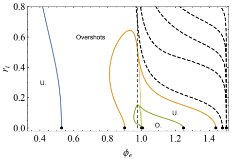
The central object is the tunneling potential $V_t(\phi)$, defined by $V_t=V-\dot\phi^2/2$; it replaces the full Euclidean profile by a one-dimensional function whose extremum gives the tunneling action. It satisfies the Euler-Lagrange equation $(4V_t'-3V')V_t'+6(V-V_t)V_t''=0$ with boundary conditions at the false vacuum and at the endpoint $\phi_0$. Pseudo-bounces are the solutions with $V_t'(\phi_e)=0$, which correspond in the Euclidean picture to a configuration with a constant inner core of radius $r_i$ and field value $\phi_e$; true bounces are the special points where $r_i=0$. The families are labeled by a parameter $A$ appearing in the low-field expansion of $V_t$, an infrared label, while $\phi_e$ and $r_i$ are ultraviolet labels; the tunneling action is a continuous function of $A$ even where $\phi_e(A)$ jumps. The relation $dS/d\phi_e=(\pi^2/2)r_i^4V'(\phi_e)$ turns the geometry of pseudo-bounce lines in the $(\phi_e,r_i)$ plane into an ordering of the actions of the bounces that they connect.
What would settle it
For the regularized example of Section 6, carry out a dense shooting scan in $A$ and in initial conditions beyond the low-field expansion, recording every endpoint where $V_t=V$ and $V_t'=0$; finding an endpoint absent from the reported branches, or any single-field potential whose number of true bounces is even, would settle that the $2n+1$ classification is incomplete.
Extended reading notes
Core claim
In the cases examined, the stationary decay configurations organize as $2n+1$ bounces: $n$ pairs each consist of one bounce and one antibounce connected by a line of pseudo-bounces, plus one extra bounce connected to a configuration of infinite radius and infinite action. A bounce has the standard shooting behavior: raising its central value produces an overshoot and lowering it produces an undershoot. An antibounce has the opposite behavior, so it is invisible or misclassified by overshoot/undershoot searches. The pseudo-bounce solutions, which have a constant inner core, trace the bottoms of valleys of the action functional in slices of fixed central field value, and the true bounces sit at the points where the core radius shrinks to zero. The authors also prove, using the relation $dS/d\phi_e=(\pi^2/2)r_i^4V'(\phi_e)$, that within each bounce-antibounce pair the configuration with the larger central field value has the lower action. These features persist after the example potentials are regularized to have finite minima, and the counting extends to an infinite family in the example with an exponential tail, where bounces and antibounces alternate with spacing tending to $\pi/\sqrt{3}$.
Load-bearing premise
The count $2n+1$ rests on the assumption that numerically integrating the tunneling-potential equation from the false vacuum with the one-parameter family $A$ sweeps out every pseudo-bounce branch; an isolated branch not reached by that family would make the claimed pairing structure incomplete.
Editorial extensions
If this is right
- Standard single-bounce codes applied to such potentials can miss the decay channel that actually dominates.
- The decay rate is not determined by the one bounce an overshoot/undershoot search finds; the relevant action can be smaller, and in the unbounded examples can even vanish.
- Within each bounce-antibounce pair the configuration at higher $\phi_e$ has lower action, so the dynamically important member of the pair is often the antibounce.
- In the exponential-tail example the infinite sequence of bounces accumulates at the singular bounce's action, so the singular bounce acts as the limit point of a spiral of ordinary decays.
- Regularizing the unbounded potentials preserves the multi-bounce structure and makes the decay action finite, so the richness is not an artifact of a runaway potential.
Reading between the lines
- A natural testable extrapolation is that the $2n+1$ valley structure appears whenever the potential has a sufficiently steep region beyond the false vacuum; a large random scan of single-field potentials would give an encounter rate for multi-bounce channels, which the paper does not attempt.
- Because $\phi_e$ and $r_i$ are ultraviolet labels, the ordering of decay channels could be sensitive to modifications of the potential at high field values even when low-energy physics is fixed; the dominant channel would then be a probe of short-distance structure.
- Appendix B's energy-conservation obstruction for spliced $V_t$ solutions suggests a general rule: one cannot lower a tunneling action by piecing together two crossing valley-bottom branches unless the splice is at the same $V_t'$, which forces the two branches to be the same solution.
Editorial analysis
A structured set of objections, weighed in public.
Referee Report
Summary. The paper studies false-vacuum decay in single-field scalar potentials using both the Euclidean bounce formalism and the tunneling potential formalism. It introduces pseudo-bounce configurations as one-parameter families labelled by the parameter A, and exhibits three example potentials in which the decay structure is far richer than the standard single bounce: Section 4 analyzes a potential from [8] with five bounces, including two 'antibounces' with reversed overshoot/undershoot behavior; Section 5 analyzes a potential from [9] with a singular bounce and an infinite sequence of bounces accumulating on it; Section 6 regularizes the first potential and shows that a finite multi-bounce structure survives. Section 7.1 states a general 2n+1 pattern for bounces, and Section 7.2 gives a Stokes' theorem proof of a relative-action inequality for bounce-antibounce pairs. The paper emphasizes that standard overshoot/undershoot codes can miss antibounce channels.
Significance. If the central claim is correct, the paper identifies a qualitatively new feature of single-field vacuum decay: the decay structure is not always described by a unique Coleman bounce, and standard searches can miss the dominant antibounce channel. The paper has several concrete strengths: the analytic bounce of Section 4 and its action are reproduced in the tunneling-potential formalism; the singular bounce of Section 5 is presented explicitly in Appendix A; the Stokes' theorem argument in Section 7.2 is a genuine analytic result that goes beyond numerical evidence; and the regularized example of Section 6 shows that the multi-bounce structure is not an artifact of unbounded-from-below potentials. However, the global 2n+1 count rests on a completeness assumption for the A-labelled pseudo-bounce family that is not proven, and the paper provides no code or numerical error estimates, so the central claim cannot currently be independently verified. These gaps temper the otherwise high potential impact of the paper.
major comments (3)
- [§4.3, Eq. (4.8); §7.1] The enumeration of bounces, and hence the abstract and §7.1 claim of exactly 2n+1 bounces, rests on the assertion in §4.3 that integrating Eq. (2.2) from the false vacuum using the low-field expansion (4.8) 'find[s] a full family of pseudo-bounces labelled by A'. This completeness is not proven. The expansion (4.8) is a one-parameter asymptotic family near ϕ=0; a second-order ODE can possess solutions whose behavior near the false vacuum is not captured by a power-log ansatz truncated at finite order. Every bounce in the paper is identified as an r_i=0 endpoint of one of these A-families, so an unproven completeness assumption is load-bearing for the central claim. The proof in §7.2 only establishes relative actions within a pair and does not address the global count. I would like to see a direct argument—for instance, a uniqueness theorem for solutions of (2.2) with the specified asymptotic behavior, or a Euclidean boundary-value count—or an explicit statement that the 2n+1 pattern is an observation from the examples rather than a proven general result.
- [Abstract; §7.1] The abstract and §7.1 claim that 'In the general case with bounce, there are 2n+1 bounces' without qualification, but the evidence consists of three concrete potentials, two of which are unbounded below and one of which has a singular bounce. Section 6 demonstrates that the 5-bounce structure of Section 4 survives a particular regularization, which is reassuring, but it is still an existence statement for a specially constructed potential. No argument is given for why a generic single-field potential with a false vacuum and a bounce must have an odd number of bounces, nor what determines n. If the intended scope is the class of potentials explored here, the wording should be revised; if the claim is meant to be universal, a proof or a precise characterization of the class of potentials is needed. As written, the paper overstates the scope of its evidence.
- [§5; Figs. 8–9] The paper reports no code, no convergence tests, and no error estimates for the numerical integrations that determine the bounce locations and actions, in particular the curves in Figures 8 and 9 for the infinite-bounce example of Section 5. The existence of an infinite sequence of bounces is supported by the analytic spiral argument, which is a strength, but the specific claim that the sequence accumulates at A≈14.7 with actions tending to S_0=130.44 is a numerical result. Similarly, the finite counts in Sections 4 and 6 depend on numerical identification of r_i=0 endpoints. For a paper whose central message is that existing numerical codes 'would miss' some decay channels, it is important that the reader can reproduce the enumeration. Please provide numerical tolerances, step sizes, and ideally the code or a clear pseudocode description.
minor comments (5)
- [§4.1, Fig. 1; §7.1] The pairing structure claimed in §7.1—that the 2n+1 bounces organize into n pairs connected by pseudo-bounce lines—is not transparent in Figure 1. The pseudo-bounce branches shown there appear to be disconnected in the (φ_e, r_i) plane (with a gap for φ_e ∈ (0.53, 0.81)), and it is unclear which bounces form the pairs. The schematic Figure 15 would be more helpful if the actual example were annotated to show the corresponding pairs.
- [§7.2, Eq. (7.3)] The proof of the relative-action inequality uses the assumption V'(φ_e)<0 to conclude the integral in (7.3) is negative. This assumption is stated only in the final step; it should be made explicit as a condition on the enclosed region A. Otherwise the statement 'Irrespective of the shape of the pseudo-bounce line' is too strong, since a potential with a local minimum inside A would have regions with V'>0 and the sign of the integral would not be fixed.
- [§5, Eq. (5.6)] The notation v_t is introduced in (5.6) as V_t(φ)=v_t(φ)e^{2φ}, but the relation between the boundary conditions (5.8) and the original tunneling-potential boundary conditions (2.3) could be stated more explicitly for readers less familiar with the formalism.
- [§4.3, last paragraph] The phrase 'cut off at φ_e=1' is vague; clarify that the cubic V_t≈−cφ^3 solution, which would otherwise run away, is terminated by the singular endpoint of the potential at φ=1, leading to a finite action that vanishes as the endpoint is approached.
- [Typographical] In §4.3, 'an spike' should be 'a spike'.
Circularity Check
No circularity: the pseudo-bounce enumeration is ODE-generated and cross-checked against Euclidean and external analytic results; the unproven completeness of the A-labeled family is a correctness caveat, not a circular reduction.
full rationale
The paper's derivations are not circular. The central enumeration of bounces, antibounces, and pseudo-bounce lines is obtained by integrating the tunneling-potential ODE (2.2) from the false vacuum with one-parameter low-field expansions (4.8)/(5.4), and then locating the endpoints satisfying V_t' = 0 or V_t' = 3V'/4; no fitted quantity is renamed as a prediction. The parameter A is explicitly called a mere label, and the action S(A) is continuous but not constructed to force the claimed 2n+1 pairing. The relative-action inequality in Sec. 7.2 follows from the identity dS/dphi_e = (pi^2/2) r_i^4 V'(phi_e), which is independently numerically checked, and from Stokes' theorem on the overshoot/undershoot boundary; it does not presuppose the conclusion. Self-citations to the tunneling-potential formalism and pseudo-bounce papers provide tools, but the examples also come from external literature ([8], [9]) and are cross-checked against Euclidean overshoot/undershoot diagrams and an external singular-bounce solution, so the self-citations are not load-bearing in the sense of an unverified premise. The strongest limitation is the unproven completeness of the A-labelled pseudo-bounce family used for the general 2n+1 statement; however, this is a numerical-completeness or extrapolation concern about correctness, not an equivalence of output to input by construction. No circular step satisfying the evidence rule is present.
Assumptions & free parameters
free parameters (3)
- phi_0 =
0.9
- phi_M =
-2.358 (tuned)
- phi_x, phi_- =
phi_x=0.975, phi_-=1.5
assumptions (4)
- domain assumption The Euclidean bounce formalism and the tunneling potential formalism are equivalent for single-field false vacuum decay (Section 2).
- domain assumption Gravity is decoupled and the field theory is four-dimensional single-field (Introduction, Sections 2 and 7.1).
- domain assumption The potentials considered have a false vacuum at phi_+ with V(phi_+)=0 and are smooth except at the stated singularities (Sections 4, 5, 6).
- ad hoc to paper The observed 2n+1 bounce pattern in the three examples is representative of the general single-field case (Section 7.1).
Cite this review
Pith. "Pith review of An Exploration of Vacuum-Decay Valleys." pith.science (2026). https://pith.science/paper/LYYK5E7R
@misc{pith2026250606154,
  author       = {Pith},
  title        = {Pith review of: An Exploration of Vacuum-Decay Valleys},
  year         = {2026},
  howpublished = {\url{https://pith.science/paper/LYYK5E7R}},
  note         = {Machine review of arXiv:2506.06154}
}
abstract
In the standard lore the decay of the false vacuum of a single-field potential is described by a semi-classical Euclidean bounce configuration that can be found using overshoot/undershoot algorithms, and whose action suppresses exponentially the decay rate. While this is generically correct, we show in a few concrete examples of potentials, previously studied in the literature for other purposes, that the vacuum decay structure can be far richer. In some cases there is no bounce and decay proceeds via the so-called pseudo-bounce configurations. In the general case with bounce, there are $2n+1$ bounces, with $n$ ranging from 0 (the standard case) to $\infty$. Some of these decay configurations we call antibounces as they have the wrong behavior for overshoot/undershoot algorithms, which can miss them. Bounce and antibounce configurations form $n$ pairs connected by pseudo-bounces. Our analysis benefits from a combined use of Euclidean and tunneling potential methods.
Figures


Figures from the paper (15 more)




Reference graph
Works this paper leans on
-
[8]
Exact tunneling solutions in multi-field potentials,
J. R. Espinosa and T. Konstandin, “Exact tunneling solutions in multi-field potentials,” JCAP03(2024), 007[hep-th/2312.12360]
arXiv 2024
-
[9]
M. Sasaki, V. Yingcharoenrat and Y. l. Zhang, “Beyond Coleman’s Instantons,” [hep-th/2411.11322]; “Singular instantons with finite action,”[hep-th/2503.19616]
-
[1]
The Fate of the False Vacuum. 1. Semiclassical Theory,
S.R. Coleman, “The Fate of the False Vacuum. 1. Semiclassical Theory,” Phys. Rev. D 15(1977) 2929 Erratum: [Phys. Rev. D16(1977) 1248]
work page 1977
-
[2]
Oscillating bounce solutions and vacuum tunneling in de Sitter spacetime,
J. C. Hackworth and E. J. Weinberg, “Oscillating bounce solutions and vacuum tunneling in de Sitter spacetime,” Phys. Rev. D71(2005) 044014[0410142/hep-th]
work page 2005
-
[4]
Standard Model vacuum decay in a de Sitter Background
A. Rajantie and S. Stopyra, “Standard Model vacuum decay in a de Sitter Background,” Phys. Rev. D97(2018) 025012[hep-th/1707.09175]
work page Pith review arXiv 2018
-
[5]
Tunneling potentials to nothing,
J. J. Blanco-Pillado, J. R. Espinosa, J. Huertas and K. Sousa, “Tunneling potentials to nothing,” Phys. Rev. D109(2024) 084057[hep-th/2311.18821]; “Bubbles of nothing: the tunneling potential approach,” JCAP03(2024) 029[hep-th/2312.00133]
arXiv 2024
-
[6]
J. R. Espinosa, “Tunneling without Bounce,” Phys. Rev. D100(2019) 105002 [hep-th/1908.01730]; J. R. Espinosa and J. Huertas, “Pseudo-bounces vs. new in- stantons,” JCAP12(2021) 029[hep-th/2106.04541]
arXiv 2019
-
[7]
A Fresh Look at the Calculation of Tunneling Actions,
J. R. Espinosa, “A Fresh Look at the Calculation of Tunneling Actions,” JCAP1807 (2018) 036[hep-th/1805.03680]
arXiv 2018
Show all 23 references
-
[10]
Fresh look at the calculation of tunneling actions including gravitational effects,
J. R. Espinosa, “Fresh look at the calculation of tunneling actions including gravitational effects,” Phys. Rev. D100(2019) 104007[hep-th/1808.00420]. 27
2019 arXiv
-
[11]
A Fresh Look at the Calculation of Tunneling Actions in Multi-Field Potentials,
J. R. Espinosa and T. Konstandin, “A Fresh Look at the Calculation of Tunneling Actions in Multi-Field Potentials,” JCAP01(2019) 051[hep-th/1811.09185]
2019 arXiv
-
[12]
The Unreasonable Effectiveness of the Tunneling Potential,
J. R. Espinosa, “The Unreasonable Effectiveness of the Tunneling Potential,” PoS CORFU2023(2024) 164[hep-th/2404.19657]
2024 arXiv
-
[13]
Instability of the Kaluza-Klein Vacuum,
E. Witten, “Instability of the Kaluza-Klein Vacuum,” Nucl. Phys. B195(1982) 481
1982
-
[14]
Catastrophic decays of compactified space-times,
M. Dine, P. J. Fox and E. Gorbatov, “Catastrophic decays of compactified space-times,” JHEP09(2004) 037[hep-th/0405190]
2004 arXiv
-
[15]
Bubble of nothing decays of unstable theories,
P. Draper, I. G. Garcia and B. Lillard, “Bubble of nothing decays of unstable theories,” Phys. Rev. D104(2021) L121701[hep-th/2105.08068]; “De Sitter decays to infinity,” JHEP12(2021) 154[hep-th/2105.10507]
2021 arXiv
-
[16]
CosmoTransitions: Computing Cosmological Phase Transition Tem- peratures and Bubble Profiles with Multiple Fields,
C. L. Wainwright, “CosmoTransitions: Computing Cosmological Phase Transition Tem- peratures and Bubble Profiles with Multiple Fields,” Comput. Phys. Commun.183 (2012) 2006[hep-ph/1109.4189]
2012 arXiv
-
[17]
Efficient numerical solution to vacuum decay with many fields,
A. Masoumi, K. D. Olum and B. Shlaer, “Efficient numerical solution to vacuum decay with many fields,” JCAP01(2017) 051[gr-qc/1610.06594]
2017 arXiv
-
[18]
Impact of Vacuum Stability Con- straints on the Phenomenology of Supersymmetric Models,
W. G. Hollik, G. Weiglein and J. Wittbrodt, “Impact of Vacuum Stability Con- straints on the Phenomenology of Supersymmetric Models,” JHEP03(2019), 109 [hep-ph/1812.04644]
2019 arXiv
-
[19]
BubbleProfiler: finding the field profile and action for cosmological phase transitions,
P. Athron, C. Bal´ azs, M. Bardsley, A. Fowlie, D. Harries and G. White, “BubbleProfiler: finding the field profile and action for cosmological phase transitions,” Comput. Phys. Commun.244(2019) 448[hep-ph/1901.03714]
2019
-
[20]
SimpleBounce : a simple package for the false vacuum decay,
R. Sato, “SimpleBounce : a simple package for the false vacuum decay,” Comput. Phys. Commun.258(2021), 107566[hep-ph/1908.10868]
2021
-
[21]
FindBounce: Package for multi-field bounce actions,
V. Guada, M. Nemevˇ sek and M. Pintar, “FindBounce: Package for multi-field bounce actions,” Comput. Phys. Commun.256(2020), 107480[hep-ph/2002.00881]
2020 arXiv
-
[22]
An optimisation based algorithm for finding the nucleation tempera- ture of cosmological phase transitions,
M. Bardsley, “An optimisation based algorithm for finding the nucleation tempera- ture of cosmological phase transitions,” Comput. Phys. Commun.273(2022), 108252 [astro-ph.CO/2103.01985]
2022 arXiv
-
[23]
BSMPT v3 A Tool for Phase Transitions and Primordial Gravitational Waves in Extended Higgs Sectors,
P. Basler, L. Biermann, M. M¨ uhlleitner, J. M¨ uller, R. Santos and J. Viana, “BSMPT v3 A Tool for Phase Transitions and Primordial Gravitational Waves in Extended Higgs Sectors,”[hep-ph/2404.19037]
-
[24]
VacuumTunneling: A package to solve bounce equation with renor- malization factor,
B. Hua and J. Zhu, “VacuumTunneling: A package to solve bounce equation with renor- malization factor,”[hep-ph/2501.15236]. 28
Reviewed August 7, 2026 · model on record in the stance chip above.
Discussion (0). Sign in to comment.