REVIEW 3 major objections 5 minor 22 references
Quadratic Extended and Unscented Kalman Filter Updates
T0 review · 3 major / 5 minor · reviewed 2026-08-07 · deepseek-v4-flash
Pith's one-line read The paper claims that replacing the linear measurement update of the Extended and Unscented Kalman Filters with a quadratic estimator that also uses the square of the measurement residual produces more accurate state estimates, with the…
desk verdict The vector-measurement update is undefined as written because P_YY is singular for m>1, so the CW results are unsupported, but the scalar case and the QUKF idea show enough merit to warrant a major revision. read the letter →
The pith
A machine-rendered reading of the paper's core claim, the machinery that carries it, and where it could break.
The reading
What carries the argument
The load-bearing object is the quadratic minimum-mean-square-error estimator and its augmented covariance block $P_{YY}$ (Eq. 22) with cross-covariance $P_{xY}$ (Eq. 21). Here $\delta y^{[2]} = \delta y \otimes \delta y$ is the Kronecker square of the measurement residual, $\mathrm{v}(P_{yy})$ is the stack operator applied to the measurement covariance, and $K = P_{xY} P_{YY}^{-1}$ acts like a Kalman gain on the augmented residual $[\delta y;\, \delta y^{[2]} - \mathrm{v}(P_{yy})]$. The argument works because the quadratic term carries third- and fourth-order moment information—skewness and kurtosis—that the linear update discards, and because both the linearization route (QEKF) and the $\sigma$-point route (QUKF) can be made to supply those moments.
What would settle it
Compute $P_{YY}$ from Eq. (22) for a two-dimensional measurement with a Gaussian prior and any nonzero measurement noise; the second block column contains identical rows for the products $\delta y_1 \delta y_2$ and $\delta y_2 \delta y_1$, so the determinant of $P_{YY}$ is identically zero. A Monte Carlo run of the Clohessy–Wiltshire example using the formulas exactly as printed would therefore fail at the inversion step, exposing that the singular case is never handled. Conversely, a run inserting a least-squares pseudo-inverse would show whether the quadratic updates still beat the linear ones once the singularity is bypassed.
Extended reading notes
Core claim
The central claim is that the linear measurement update shared by the EKF and UKF is the reason these filters leave accuracy on the table, and that a modest modification—replacing the linear estimator $g_L(y)$ with the parabolic $g_Q(y) = \mathbb{E}[x] + B\, \delta y + C\, \delta y^{[2]}$—recovers part of the nonlinear conditional mean. The optimal constants $B^*$ and $C^*$ follow from the orthogonality principle: they are the augmented Kalman gain $K = P_{xY} P_{YY}^{-1}$, where the augmented matrices contain cross-covariances with $\delta y^{[2]}$ and the covariance of $\delta y^{[2]}$ itself, offset by $\mathrm{v}(P_{yy})$. The QEKF evaluates these moments by linearizing the measurement model and applying Isserlis' formula for Gaussian kurtosis, while the QUKF evaluates them by propagating $\sigma$ points and their Kronecker squares. The update equations retain the familiar Kalman form, with the residual vector augmented by $\delta y^{[2]} - \mathrm{v}(P_{yy})$.
Load-bearing premise
The update rule requires the augmented covariance matrix $P_{YY}$ to be invertible, but for any measurement of dimension greater than one the measurement-square vector contains duplicate entries, so $P_{YY}$ is singular and the inverse in the gain formula does not exist as written.
Editorial extensions
If this is right
- For nonlinear measurement models or non-Gaussian measurement noise, the quadratic update should systematically beat the corresponding linear filter, since a parabola can bend toward the conditional mean where a straight line cannot.
- Because the update formulas are written in terms of moments only, they transfer directly to other linear estimators such as the Cubature, Central Difference, and Ensemble Kalman Filters, upgrading them to quadratic versions without changing their prediction steps.
- The added computational cost is small relative to particle or Gaussian-sum filters, since only an augmented covariance of dimension $m + m^2$ needs to be built and inverted at each step.
- Generalizing the same derivation to cubic and higher polynomial residuals should continue improving accuracy, trending toward the true MMSE estimator as the polynomial order grows.
Reading between the lines
- The paper leaves unsigned the fact that $\delta y \otimes \delta y$ duplicates entries whenever the measurement dimension $m$ exceeds 1 (e.g., $\delta y_1 \delta y_2$ and $\delta y_2 \delta y_1$ are identical), making the augmented covariance $P_{YY}$ singular by construction and the gain $P_{xY} P_{YY}^{-1}$ undefined as written; a pseudo-inverse, a de-duplication to $m(m+1)/2$ terms, or a small
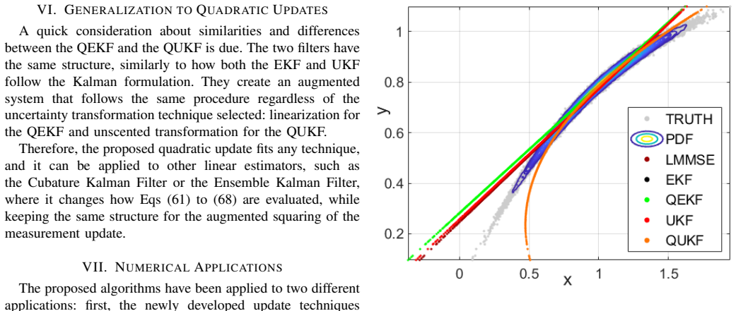
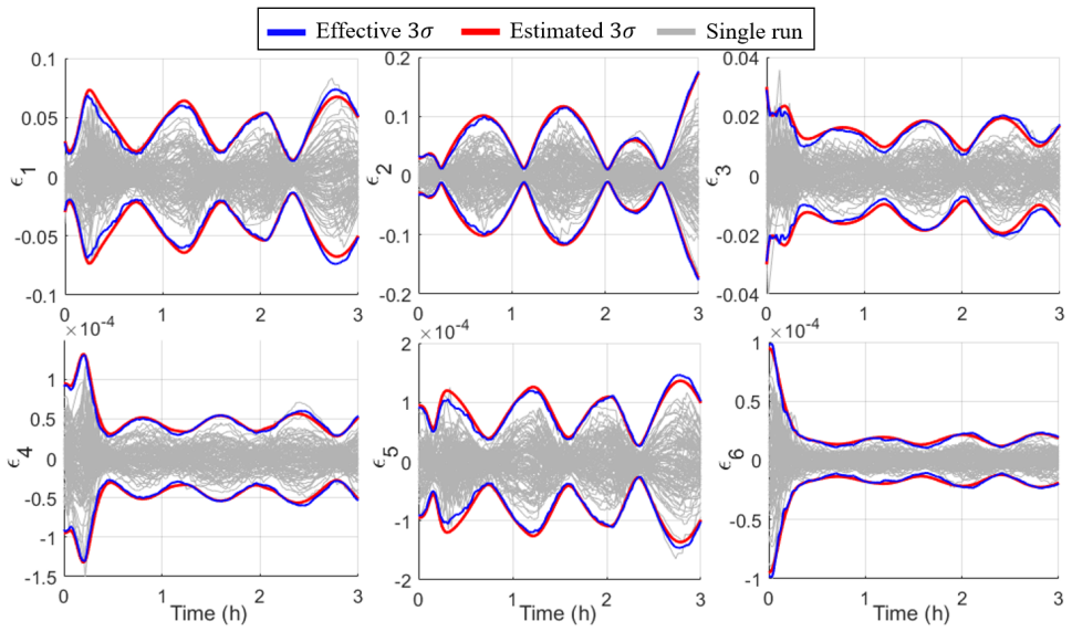
- The claimed ~25% improvement is measured only in the scalar example; the Clohessy–Wiltshire experiment shows lower error qualitatively but does not report a comparable error reduction, so the size of the benefit in realistic problems remains open.
- The paper's scalar comparison also shows QEKF reducing to EKF under a Gaussian prior; an interesting test would be to run QEKF with a genuinely skewed prior to see whether a linearization-based quadratic update can match the sigma-point-based one.
- A consistency check in the rank-deficient case would be whether the update $P_{xx}^+ = P_{xx}^- - K P_{YY} K^T$ remains symmetric positive semidefinite when $P_{YY}$ is pseudo-inverted.
Editorial analysis
A structured set of objections, weighed in public.
Referee Report
Summary. The paper proposes quadratic extensions of the extended and unscented Kalman filters. The authors derive a quadratic MMSE estimator from the orthogonality principle, with the update g(y) = E[x] + B(y-E[y]) + C((y-E[y])⊗(y-E[y]) - vec(P_yy)). They compute the required moments using linearization (QEKF) and the unscented transform (QUKF), and evaluate the filters on a scalar toy problem and on a Clohessy-Wiltshire relative-navigation problem with two angle measurements. The paper claims that these quadratic updates outperform their linear counterparts and that the formulation can be generalized to other linear estimators.
Significance. The idea of upgrading linear Kalman updates with quadratic terms is of practical interest, and the derivation is self-contained and mostly clear. The scalar experiment shows a meaningful RMSE improvement for the QUKF, and the method, if valid for vector measurements, could be applied to other filters such as CKF and EnKF. However, the vector-measurement case is not well defined as written, and the main numerical application is affected. The paper's claims are therefore only partially supported.
major comments (3)
- [Section II, Eqs. (20)-(23) and Section VII-B] For measurement dimension m>1, the augmented covariance matrix P_YY in Eq. (22) is singular by construction. The vector δy[2]=δy⊗δy contains identical products (e.g., δy_1 δy_2 and δy_2 δy_1), so there exist nonzero vectors e such that the linear combination e^T[δy; δy[2]] is identically zero. Therefore e^T P_YY e = 0, and P_YY^{-1} in Eqs. (20), (23), and (34) does not exist. The subtraction of v(P_yy)v(P_yy)^T in the lower-right block does not remove this degeneracy. Since the Clohessy-Wiltshire experiment in Section VII-B uses a two-dimensional measurement vector (Eqs. (77)-(78)), the central numerical claim cannot be reproduced from the equations as written. The paper notes that earlier polynomial updates were restricted to scalar measurements because of matrix singularity (Section I), but it does not propose a pseudo-inverse, regularization, or a reduced set of unique quadratic monomials.
- [Section VII-A and Section VIII] The scalar example does not support the claimed benefits for QEKF: because the prior is Gaussian and the Isserlis assumption (Eqs. (45)-(46)) is used, S_xxx=0 and hence P_xy[2]=0 (Eq. (39)), so the QEKF update in Eq. (35) reduces to the EKF update. In Fig. 2 the QEKF and EKF bars are identical. Thus the only valid demonstration of a quadratic improvement is the QUKF in the scalar example and the (undefined) vector example. The conclusion in Section VIII that 'the QEKF and QUKF propose significant improvements' is therefore not supported for QEKF by the presented evidence.
- [Section IV, Eq. (36)] If a pseudo-inverse of P_YY were used to repair the vector case, the covariance update P_xx^+ = P_xx^- - K P_YY K^T would require additional justification. For a rank-deficient regressor, the minimum-norm solution of the normal equations does not in general give the posterior covariance of the resulting estimator; the error covariance of the quadratic estimator differs from this expression unless the regressor covariance is nonsingular. The paper does not provide such a justification.
minor comments (5)
- [Eq. (19)] The right-hand side as typeset appears to be [P_xy P_xy[2]]^T, but the product [B* C*] P_YY is an n_x × (m+m^2) matrix; the right-hand side should be [P_xy P_xy[2]] (without transpose). Please correct the notation.
- [Section II, final paragraph] The phrase 'the Quadratic Unscented Kalman Filter (UKF)' should read '(QUKF)'.
- [Eq. (60)] The symbol δY is used both for the measurement deviation Y_k^{(i)} - y_k and for the augmented deviation that includes the Kronecker square; using a separate symbol (e.g., δY_aug) would avoid ambiguity.
- [Figure 5 caption] The word 'respectfully' should be 'respectively'.
- [Section VII-B] Please state explicitly whether the two measurement noises η1 and η2 are mutually independent and independent over time, as this is used implicitly in the covariance expressions (Eqs. (66)-(68)).
Circularity Check
No significant circularity: the QMMSE update is derived self-contained from the orthogonality principle; self-citations are contextual, not load-bearing. A separate well-posedness flaw affects the vector-measurement update.
full rationale
The central derivation is self-contained. The paper starts from the standard orthogonality condition E[(x - g_Q*(y)) g_Q(y)^T] = 0 (Eq. 5), substitutes the three test estimators (Eqs. 6-9), obtains the normal equations (Eqs. 10-11), assembles them into the augmented linear system (Eq. 19), solves for K = P_xY P_YY^{-1} (Eq. 20), and substitutes back to obtain the quadratic estimator g_Q*(y) = E[x] + P_xY P_YY^{-1} [δy; δy[2] - v(P_yy)] (Eq. 23). No parameter is fitted to the reported test data and then renamed a prediction; the gains B* and C* are computed from prior moments, via linearization for the QEKF and sigma points for the QUKF. The reported accuracy improvements, including the roughly 25% scalar RMSE improvement, are therefore an honest consequence of enlarging the estimator family rather than a circular fit. The self-citations ([19], [20], [22]) provide context and elementary tensor identities (e.g., S_xxx = P_x[2]x and K_xxxx = P_x[2]x[2] for null-mean distributions), but the derivation does not reduce to those citations. Separately, the paper itself acknowledges that prior polynomial updates were 'tested only with scalar measurements, avoiding the issue of matrix singularity'; the present formulation has the same by-construction singularity for any vector measurement, because δy[2] = δy⊗δy contains duplicated entries for m > 1, making P_YY in Eq. (22) singular and P_YY^{-1} in Eqs. (20), (23), and (34) nonexistent as written. The Clohessy-Wiltshire example uses a two-dimensional measurement vector, so that numerical claim is not reproducible from the stated equations. This is a correctness and well-posedness concern, not a circularity concern, and it is reflected here only by not raising the circularity score above 2. The score of 2 reflects the cluster of non-load-bearing self-citations, not any actual circular derivation.
Assumptions & free parameters
free parameters (1)
- UKF scaling parameters α, β, κ =
not reported
assumptions (4)
- standard math Orthogonality principle characterizes the optimal quadratic estimator (Eqs. 5-23).
- domain assumption Measurement noise moments (covariance, skewness, kurtosis) are exactly known and noise is independent of state.
- ad hoc to paper State prior skewness and kurtosis are available; for a Gaussian prior, S_xxx=0 and K_xxxx follows Isserlis' formula (Eqs. 45-46).
- ad hoc to paper The augmented covariance P_YY is nonsingular and its inverse in Eqs. 20 and 34 exists.
Cite this review
Pith. "Pith review of Quadratic Extended and Unscented Kalman Filter Updates." pith.science (2026). https://pith.science/paper/JPMPL4ZO
@misc{pith2026250606256,
  author       = {Pith},
  title        = {Pith review of: Quadratic Extended and Unscented Kalman Filter Updates},
  year         = {2026},
  howpublished = {\url{https://pith.science/paper/JPMPL4ZO}},
  note         = {Machine review of arXiv:2506.06256}
}
read the original abstract
Common filters are usually based on the linear approximation of the optimal minimum mean square error estimator. The Extended and Unscented Kalman Filters handle nonlinearity through linearization and unscented transformation, respectively, but remain linear estimators, meaning that the state estimate is a linear function of the measurement. This paper proposes a quadratic approximation of the optimal estimator, creating the Quadratic Extended and Quadratic Unscented Kalman Filter. These retain the structure of their linear counterpart, but include information from the measurement square to obtain a more accurate estimate. Numerical results show the benefits in accuracy of the new technique, which can be generalized to upgrade other linear estimators to their quadratic versions.
Figures


Figures from the paper (2 more)

Reference graph
Works this paper leans on
-
[2]
Gelbet al.,Applied optimal estimation
A. Gelbet al.,Applied optimal estimation. MIT press, 1974
1974
-
[1]
A new approach to linear filtering and prediction problems,
R. E. Kalman, “A new approach to linear filtering and prediction problems,” 1960
1960
-
[3]
How nonlinear is it? a tutorial on nonlin- earity of orbit and attitude dynamics,
J. L. Junkins and P. Singla, “How nonlinear is it? a tutorial on nonlin- earity of orbit and attitude dynamics,”The Journal of the Astronautical Sciences, vol. 52, pp. 7–60, 2004
work page 2004
-
[4]
Unscented filtering and nonlinear estimation,
S. J. Julier and J. K. Uhlmann, “Unscented filtering and nonlinear estimation,”Proceedings of the IEEE, vol. 92, no. 3, pp. 401–422, 2004
2004
-
[5]
I. Arasaratnam and S. Haykin, “Cubature kalman filters,”IEEE Trans- actions on automatic control, vol. 54, no. 6, pp. 1254–1269, 2009
work page 2009
-
[6]
Differential algebra-based multiple gaussian particle filter for orbit determination,
S. Servadio and R. Zanetti, “Differential algebra-based multiple gaussian particle filter for orbit determination,”Journal of Optimization Theory and Applications, vol. 191, no. 2, pp. 459–485, 2021
work page 2021
-
[7]
A gaussian particle filter based on differential algebra for spacecraft navigation,
M. Valli, R. Armellin, P. Di Lizia, and M. Lavagna, “A gaussian particle filter based on differential algebra for spacecraft navigation,” 2012
work page 2012
-
[8]
A finite-difference method for linearization in nonlinear estimation algorithms,
T. S. Schei, “A finite-difference method for linearization in nonlinear estimation algorithms,”Automatica, vol. 33, no. 11, pp. 2053–2058, 1997
work page 1997
Show all 22 references
-
[9]
A high order method for estimation of dynamic systems,
M. Majji, J. L. Junkins, and J. D. Turner, “A high order method for estimation of dynamic systems,”The Journal of the Astronautical Sciences, vol. 56, no. 3, pp. 401–440, 2008
2008
-
[10]
Nonlinear mapping of uncertainties in celestial mechanics,
M. Valli, R. Armellin, P. Di Lizia, and M. R. Lavagna, “Nonlinear mapping of uncertainties in celestial mechanics,”Journal of Guidance, Control, and Dynamics, vol. 36, no. 1, pp. 48–63, 2013
2013
-
[11]
Recursive bayesian estimation using gaussian sums,
H. W. Sorenson and D. L. Alspach, “Recursive bayesian estimation using gaussian sums,”Automatica, vol. 7, no. 4, pp. 465–479, 1971
1971
-
[12]
Nonlinear bayesian estimation using gaussian sum approximations,
D. Alspach and H. Sorenson, “Nonlinear bayesian estimation using gaussian sum approximations,”IEEE transactions on automatic control, vol. 17, no. 4, pp. 439–448, 2003
2003
-
[13]
Novel approach to nonlinear/non-gaussian bayesian state estimation,
N. J. Gordon, D. J. Salmond, and A. F. Smith, “Novel approach to nonlinear/non-gaussian bayesian state estimation,” inIEE proceedings F (radar and signal processing), vol. 140, pp. 107–113, IET, 1993
1993
-
[14]
The gaussian particle filter for diagnosis of non-linear systems,
F. Hutter and R. Dearden, “The gaussian particle filter for diagnosis of non-linear systems,”IF AC Proceedings V olumes, vol. 36, no. 5, pp. 909– 914, 2003
2003
-
[15]
Likelihood scouting via map inversion for a posterior- sampled particle filter,
S. Servadio, “Likelihood scouting via map inversion for a posterior- sampled particle filter,”IEEE Transactions on Aerospace and Electronic Systems, 2024
2024
-
[16]
Optimal quadratic fil- tering of linear discrete-time non-gaussian systems,
A. De Santis, A. Germani, and M. Raimondi, “Optimal quadratic fil- tering of linear discrete-time non-gaussian systems,”IEEE Transactions on Automatic Control, vol. 40, no. 7, pp. 1274–1278, 1995
1995
-
[17]
Polynomial filtering of discrete-time stochastic linear systems with multiplicative state noise,
F. Carravetta, A. Germani, and N. Raimondi, “Polynomial filtering of discrete-time stochastic linear systems with multiplicative state noise,” IEEE Transactions on Automatic Control, vol. 42, no. 8, pp. 1106–1126, 1997
1997
-
[18]
Polynomial extended kalman filter,
A. Germani, C. Manes, and P. Palumbo, “Polynomial extended kalman filter,”IEEE Transactions on Automatic Control, vol. 50, no. 12, pp. 2059–2064, 2005
2005
-
[19]
Recursive polynomial minimum mean- square error estimation with applications to orbit determination,
S. Servadio and R. Zanetti, “Recursive polynomial minimum mean- square error estimation with applications to orbit determination,”Journal of Guidance, Control, and Dynamics, vol. 43, no. 5, pp. 939–954, 2020
2020
-
[20]
Nonlinear filtering with a polynomial series of gaussian random variables,
S. Servadio, R. Zanetti, and B. A. Jones, “Nonlinear filtering with a polynomial series of gaussian random variables,”IEEE Transactions on Aerospace and Electronic Systems, vol. 57, no. 1, pp. 647–658, 2020
2020
-
[21]
On a formula for the product-moment coefficient of any order of a normal frequency distribution in any number of variables,
L. Isserlis, “On a formula for the product-moment coefficient of any order of a normal frequency distribution in any number of variables,” Biometrika, vol. 12, no. 1/2, pp. 134–139, 1918
1918
-
[22]
Estimation of the conditional state and covariance with taylor polynomials,
S. Servadio and R. Zanetti, “Estimation of the conditional state and covariance with taylor polynomials,”Journal of Advances in Information Fusion, vol. 16, no. 2, p. 126, 2021. 8
2021
Reviewed August 7, 2026 · model on record in the stance chip above.
Discussion (0). Sign in to comment.