Stochastic Gradient-Descent Calibration of Pyragas Delayed-Feedback Control for Chaos Suppression in the Sprott Circuit

Adib Kabir; Caitlin Hult; Juthi Hira; Oishi Kabir; Onil Morshed

REVIEW 4 major objections 6 minor 17 references

Stochastic Gradient-Descent Calibration of Pyragas Delayed-Feedback Control for Chaos Suppression in the Sprott Circuit

T0 review · 4 major / 6 minor · reviewed 2026-08-07 · deepseek-v4-flash

Challenge this review Re-run · record.json Download PDF Read on arXiv ↗

Pith's one-line read Stochastic gradient descent with finite differences can calibrate delayed-feedback chaos control on the Sprott circuit, aligning simulated and digitized experimental waveforms in phase and amplitude better than grid-search SSE.

desk verdict A modest calibration study whose central claim—SGD beats grid search for this Pyragas-control problem—is not supported by the reported numbers; the optimizer lands on its own bounds and no loss values are given. read the letter →

arxiv 2506.06639 v2 pith:JROCE6SZ submitted 2025-06-07 nlin.CD math.OCphysics.comp-ph

Adib Kabir , Onil Morshed , Oishi Kabir , Juthi Hira , Caitlin Hult This is my paper

classification nlin.CDmath.OCphysics.comp-ph MSC 37D4534C2893C10 PACS 05.45.-a05.45.Gg

keywords SprottcircuitPyragasdelayedfeedbackcontrolstochasticgradientdescentchaossuppressionparametercalibrationsumofsquarederrorsfinite-differencephasesynchronization

verification ladder T0 review T1 audit T2 compute T3 formal

The pith

A machine-rendered reading of the paper's core claim, the machinery that carries it, and where it could break.

The reading

This paper claims that stochastic gradient descent (SGD), with gradients estimated by finite differences, can calibrate a Pyragas delayed-feedback controller for the Sprott chaotic circuit more effectively than the standard grid-search sum-of-squared-errors method. The calibration tunes three parameters jointly: feedback gain K, delay time Tcon, and circuit resistor Rv. Against a target waveform of 284 voltage points manually digitized from a published experiment, the jointly tuned simulation aligns with the experimental trace in both phase and amplitude, where grid-search calibration leaves a persistent phase drift. If correct, this means a first-order optimizer can replace exhaustive grid searches for controlling and modeling chaotic circuits, even when analytic gradients are unavailable. The paper also shows that tuning the physical resistor Rv, not just the control parameters, is what removes most of the mismatch.

What carries the argument

The mechanism carrying the argument is the Pyragas delayed-feedback control signal u(τ) = sat(K(x1(τ − Tcon) − x1(τ))) added to the third-order Sprott circuit ODE, combined with a loss function that sums squared errors in both the capacitor voltage and the control signal. Since no analytic gradients are available, the optimizer estimates ∂J/∂T, ∂J/∂K, and ∂J/∂Rv by finite differences (with ε = $10^{-3}$ for T and K, and a scaled step for Rv), then applies the standard SGD update θ ← θ − α∇J with learning rate α = 0.01. The state-space formulation (x1 = x, x2 = −ẋ, x3 = ẍ) integrated with a fourth-order Runge-Kutta method at Δτ = 0.01 is what turns the differential equation into a simulator for the loss landscape. The key structural fact is that adding Rv as a free parameter raises the number of simulations per gradient step from 4 to 6, and this extra degree of freedom is what lets the optimizer absorb structural mismatch between model and experiment.

What would settle it

Take raw experimental voltage traces from a Sprott circuit under Pyragas control, with calibrated time base and error bars. If the SGD-optimized (Tcon, K, Rv) = (7.0, 0.25, 100 kΩ) simulation does not track those traces better than the grid-search result, or if synthetic-data tests with known parameters fail to recover them, the central claim fails. Concretely, one could run the same finite-difference SGD on a dataset generated from the model with parameters inside the allowed ranges; successful recovery within tolerance would support the method, while convergence to boundary values or wrong parameters would falsify the claim that SGD calibrates the controller.

Watch

Extended reading notes

Core claim

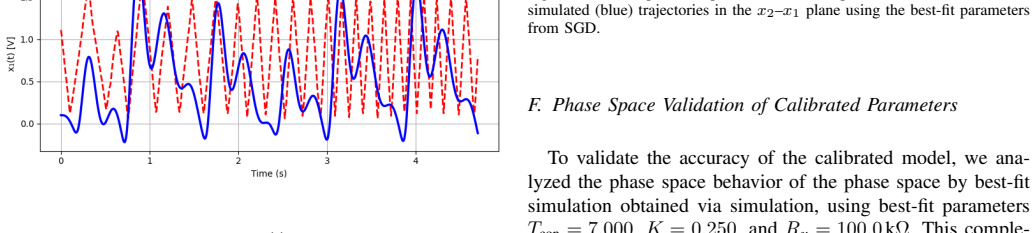
The central claim the paper argues for is that joint SGD optimization of the control parameters and a physical circuit parameter reaches a qualitatively better fit than optimizing control parameters alone or via grid search. Concretely, with Tcon = 7.000, K = 0.250, and Rv = 100.0 kΩ, the simulated capacitor voltage x1(t) tracks the digitized experimental waveform in amplitude and phase, reproducing peak sharpness and frequency content; the phase-space portrait in the x2–x1 plane also matches the experimental attractor's overall loop geometry. The authors attribute this improvement to expanding the optimization from a two-parameter control space (Tcon, K) to a three-parameter space that includes Rv. They present this as evidence that SGD-based calibration is a viable path for precise control of chaotic electronic systems.

Load-bearing premise

The load-bearing premise is that the 284-point experimental waveform manually digitized from published figures is accurate enough to serve as ground truth for calibration; all fitted parameters and all accuracy comparisons inherit whatever systematic errors that digitization introduced.

Editorial extensions

If this is right

If SGD calibration works as claimed, chaotic circuit models can be fitted to experimental voltage traces without analytic gradients, using only repeated simulation and finite differences.
Jointly calibrating physical parameters such as Rv alongside control parameters becomes the recommended practice, since fixing them leaves phase drift and amplitude mismatch.
The demonstrated fit implies that a three-parameter SGD calibration can serve as a benchmark for comparing control strategies on the Sprott circuit, with phase synchronization as a meaningful quality metric.
The computational cost model Nsim = 2d · E gives a concrete scaling law: each added parameter adds two simulations per SGD iteration, so calibration cost grows linearly with parameter dimension.

Reading between the lines

Editorial extensions of the paper, not claims the author makes directly.

Because the experimental reference is 284 manually digitized points with acknowledged systematic errors, the quantitative superiority of SGD over grid search should be read as provisional; a re-test against raw voltage data with time-base calibration would be the decisive check.
The reported optimum sits at the boundary of the parameter clips (Tcon = 7.0, K = 0.25, Rv = 100 kΩ), so part of the improvement may come from the chosen bounds rather than from gradient-driven convergence; checking interior solutions or wider ranges would clarify.
The loss includes a term comparing simulated and experimental control signals, but experimental u(t) is not measured independently; if u_exp is reconstructed from the model, the loss partly measures the model against itself.
A natural extension would be to use the same finite-difference SGD pipeline on synthetic data generated from known parameters, which would isolate optimization performance from digitization noise.

Share X Bluesky LinkedIn Reddit HN

Editorial analysis

A structured set of objections, weighed in public.

Desk editor's note, referee report, and a circularity audit.

Desk Editor's Note

read the letter

Colleague,

This is a modest engineering study: apply SGD with finite-difference gradients to tune three parameters (delay, gain, Rv) of a Pyragas-controlled Sprott circuit model, comparing against a grid-search baseline. The paper is honest about its data limitations and includes a phase-space check, a computational-cost analysis, and a code link. Credit where due: the authors clearly state that the experimental target is 284 points manually digitized from published figures, that this introduces systematic errors, and that raw data were unavailable. That's refreshing.

The problem is the central quantitative comparison. The claims that joint SGD 'aligns well in amplitude and phase' and is 'better than grid search' rest on visual inspection of one waveform. No SSE values, loss curves, or convergence plots are reported. Worse, the fitted parameters in Figure 11 are Tcon=7.000, K=0.250, Rv=100.0 kΩ—exactly the upper bounds in Algorithm 1. That is not evidence of convergence to an interior optimum; it is the optimizer hitting the edge of the allowed box. You cannot tell whether the gradient is still pointing outward or whether the true optimum lies outside.

The comparison is also not apples-to-apples. The grid search ran over Tcon ∈ [1.5,2.5], K ∈ [0.8,1.5], while the SGD ran over Tcon ∈ [6,7], K ∈ [0.05,0.25] plus Rv. These parameter ranges barely overlap, so beating a grid search that was restricted to a different, largely disjoint region is not meaningful.

There's a second internal inconsistency: the loss in Eq. (9) includes a term Σ(u_sim - u_exp)², but only x1(t) is digitized. No experimental control signal is described, plotted, or deposited. If u_exp is silently zero, the loss penalizes any nonzero control, which conflicts with the nonzero optimal K. If it's not zero, its provenance is missing. Either way the objective is ambiguous.

Minor: the label 'stochastic' is unsupported—the algorithm uses the full batch of 284 points, no mini-batching. The code link has no commit hash and the data are 'available upon request', so the results are not reproducible as described.

In balance: the paper is a reasonable exercise but the load-bearing claim is not backed by the reported evidence. It deserves a serious referee—there is enough substance and honesty to warrant expert review—but I expect rejection unless the authors supply loss values, re-run the grid search over a comparable parameter space, and clarify the u_exp term. Not something I'd cite.

Referee Report

4 major / 6 minor

Summary. This manuscript presents a numerical calibration study of Pyragas delayed-feedback control for the Sprott circuit. The authors integrate the third-order model of Merat et al., digitize 284 points of the capacitor voltage x1(t) from published figures using WebPlotDigitizer, and minimize the sum of squared errors against this target using grid search over (Tcon, K) and SGD with finite-difference gradients over (Tcon, K, Rv). They report that joint SGD calibration produces the best amplitude and phase alignment, and they use phase-space plots to argue that the calibrated model reproduces the experimental attractor geometry. The paper concludes that SGD-based calibration shows significant potential for precise control of chaotic systems.

Significance. If the central quantitative claim were supported, the paper would offer a modest methodological demonstration: a first-order finite-difference optimizer can tune three parameters of a known chaotic circuit model to match a digitized experimental trace. The manuscript is candid about its data-extraction limitations and provides a code repository link in the supplementary material, which is a strength. However, the claimed advantage over grid search is not backed by any reported loss value, convergence diagnostic, or uncertainty estimate, and the objective function as written is not fully defined because the experimental control signal u_exp is never specified. The result is therefore not yet a reliable evidence point for SGD-based calibration in this setting.

major comments (4)

[§IV.E, Fig. 11, Algorithm 1] The headline result is a boundary artifact. Algorithm 1 clamps Tcon to [6.0, 7.0], K to [0.05, 0.25], and Rv to [60, 100] kΩ, and the best-fit parameters reported in Fig. 11 are exactly Tcon = 7.000, K = 0.250, Rv = 100.0 kΩ. No loss values or convergence curves are given for any SGD run, so it is impossible to tell whether the optimizer converged to an interior minimum or simply ran into the upper edge of the feasible box. Because the central claim of §IV.E is that joint SGD is quantitatively better than grid search, the manuscript must report final loss values, per-parameter trajectories, and behavior at the bounds; better, it should use bounds wide enough that the optimum is interior.
[§III.C, Eq. (9)] Eq. (9) defines the SGD objective as a voltage SSE plus a control-signal SSE over u_sim and u_exp, but the paper never describes, plots, or deposits any experimental control signal u_exp; Section III.A only digitizes the x1(t) voltage trace. If u_exp is absent, the second term cannot be evaluated; if it is silently set to zero, the term penalizes any nonzero control signal, which conflicts with the optimized gain K = 0.25. This makes the objective undefined or self-contradictory as reported. The authors should either remove the u term from the loss and state exactly which loss was used, or provide the u_exp dataset used.
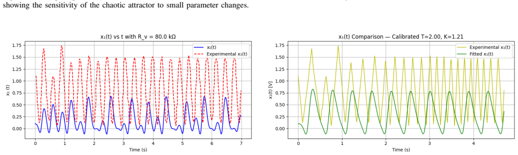
[§III.B, §IV.D, §IV.E] The comparison between grid search and SGD is not apples-to-apples. Grid search is run over Tcon ∈ [1.5, 2.5] and K ∈ [0.8, 1.5] using the loss in Eq. (7), while SGD is run over Tcon ∈ [6, 7], K ∈ [0.05, 0.25], plus Rv, using the different loss in Eq. (9). The parameter ranges have almost no overlap and the objectives differ, so the visual superiority of Fig. 11 over Fig. 9 cannot be attributed to the optimization method rather than to the different search space or loss. Both methods need to be compared on the same objective and an overlapping parameter domain.
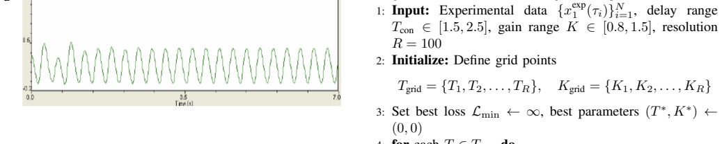
[§III.A, Fig. 3, §V] The calibration target is a manually digitized trace of 284 points with acknowledged systematic errors, and no raw extracted data, uncertainty bars, or timing calibration are provided. Every fitted parameter and every claimed improvement is measured against this target, so the 'phase-space validation' in §IV.F is not an independent test but a check of the fitted trajectory against the same data source. To support the validation language, the authors should deposit the extracted dataset, quantify digitization uncertainty by re-digitizing the figures multiple times, and report an out-of-sample or independent metric such as Lyapunov exponents or a held-out portion of the time series.

minor comments (6)

[§IV.D] The text refers to 'Section III.A' for the SSE calibration method, but the method is described in Section III.B; this cross-reference should be corrected.
[Figs. 1 and 2] Figures 1 and 2 appear as placeholder asterisks and are not referenced in the text; they should either be removed or replaced with actual figures.
[§II, Eq. (6)] The nonlinear term is written as D(x) in Eq. (1) and as D(x1) in Eq. (6), while Section VI refers to a diode function u(x); the notation should be made consistent throughout.
[§IV.G] The text says the simulation count grows 'from 400 to 6000' across 100 epochs, but the formula Nsim = 2dE gives 400 for d = 2 and 600 for d = 3; Appendix A correctly states 600. This arithmetic error should be fixed.
[Appendix A, §IV.F] Phrases such as 'orders like orders' and 'the order's validity' are garbled; these should be rewritten as 'attractor' or 'model' as appropriate.
[§III.C] The method is called stochastic gradient descent, but the described finite-difference procedure appears to use the full 284-point dataset and no mini-batching; the authors should either specify the stochastic sampling scheme or call the method (full-batch) gradient descent.

Circularity Check

1 steps flagged · score 4.0 of 10

Partial circularity: the phase-space 'validation' is an in-sample re-plot of the fitted simulation against the same digitized data used to build the loss, so the central support for SGD superiority reduces to reporting the training fit.

fitted input called prediction [Section IV-F (Phase Space Validation), Fig. 12; loss defined in Eq. (9) in Section III-C]
"To validate the accuracy of the calibrated model, we analyzed the phase space behavior of the phase space by best-fit simulation obtained via simulation, using best-fit parameters Tcon = 7.000, K = 0.250, and Rv = 100.0 kΩ. This complements the time-domain comparison by evaluating whether the simulated trajectory correctly reproduces the geometry of the experimental attractor in the x2–x1 plane."

The parameters Tcon=7.000, K=0.250, Rv=100.0 kΩ are the result of minimizing the SSE loss J(T,K,Rv) = Σ(x_sim1 − x_exp1)^2 + Σ(u_sim − u_exp)^2 (Eq. 9) against the same 284 digitized experimental points described in Section III-A. The 'validation' phase portrait is generated from this same fitted simulation and compared with the experimental attractor extracted from the same published figures (Fig. 3f) used to build the loss. Therefore the phase-space agreement is not an independent check: it is a re-plot of the training fit. The claim that the phase-space analysis 'validates' the model reduces to reporting the in-sample fit, so the validation is statistically forced by the fitting procedure rather than being an out-of-sample prediction.

full rationale

The paper's core derivation chain is largely external and not circular: the Sprott-circuit model, the Pyragas delayed-feedback law, and the saturation function are all taken from prior published work (Merat et al. and Pyragas), not from the authors' own self-citations, and the numerical integration is a standard RK4 implementation. No uniqueness theorem or ansatz is smuggled in via self-citation, and the code is publicly provided. The circularity that does exist is the same-data validation pattern. The loss functions in Eqs. (7) and (9) are defined as the squared error between simulated and digitized experimental x1(t), and the reported 'best' parameters are the minimizers of that loss. Section IV-F then presents a phase-space comparison using those same fitted parameters and the same digitized experimental figures as a 'validation' of the model. That is not a prediction of new or held-out behavior; it is a graphical restatement of the training fit, which is why the phase-space agreement is forced by construction to be the best available in-sample alignment. The additional weaknesses noted by the skeptical reading — the SGD optimum sitting exactly on all three upper bounds, the non-overlapping grid-search and SGD parameter ranges, and the undefined experimental control signal u_exp in Eq. (9) — are serious correctness and reproducibility concerns, but they are not themselves circularity, so they do not raise the score beyond 4. The central quantitative claim would need held-out data, reported loss curves, or an independent experimental comparison to escape this partial circularity.

Assumptions & free parameters 3 free parameters · 4 assumptions · 1 invented entities

The central claim rests on three fitted parameters (Tcon, K, Rv) plus the inherited Merat ODE and the digitized data treated as ground truth. The only new object is the SGD calibration procedure itself, which is standard and does not invent new physics.

free parameters (3)

Tcon (delay) = 2.00 (grid), 7.000 (SGD fixed Rv), 7.000 (SGD joint)
Fitted to digitized experimental data via SSE grid search and SGD; the SGD value sits exactly on the algorithm's upper clip bound.
K (gain) = 1.21 (grid), 0.050 (SGD fixed Rv), 0.250 (SGD joint)
Fitted to digitized experimental data; the SGD fixed-Rv value sits on the lower clip bound and the joint value on the upper clip bound, indicating boundary saturation.
Rv (variable resistor) = 80.0 kOhm fixed in SSE and fixed-Rv SGD; 100.0 kOhm in joint SGD
Treated as fixed circuit parameter from Merat et al. in two calibrations, then fit by SGD in the joint calibration; the fitted value equals the upper clip bound.

assumptions (4)

domain assumption The Merat et al. third-order ODE (Eq. 1) with the piecewise-linear diode D(x) = -min(R2/R1 x, 0) accurately describes the experimental Sprott circuit.
The entire calibration inherits this model without independent validation. Section II states the paper 'adopts' Eq. (1) from [1].
domain assumption Digitized points from published figures, after WebPlotDigitizer extraction, are a faithful time-aligned representation of the experimental voltage x1(t).
Section III-A describes the extraction and explicitly notes 'systematic errors' and 'cumbersome data plotting task'.
domain assumption The Pyragas control form (Eqs. 3-5) with the stated saturation limits is the correct model of the experimental controller.
Section II adopts u(t) = sat(K(x1(t-Tcon)-x1(t))) + u0 from Merat et al. [1].
standard math A fixed-step RK4 integration of the ODE accurately represents the true continuous dynamics for the simulated trajectories.
Section III-B states RK4 with fixed dt = 0.01 without convergence checks or error control.

invented entities (1)

None
purpose: N/A
The paper does not introduce new physical entities, particles, forces, or dimensions. Its contribution is purely a parameter-calibration comparison on an existing model.

how reviews work

0 comments

Cite this review

Pith. "Pith review of Stochastic Gradient-Descent Calibration of Pyragas Delayed-Feedback Control for Chaos Suppression in the Sprott Circuit." pith.science (2026). https://pith.science/paper/JROCE6SZ

@misc{pith2026250606639,
  author       = {Pith},
  title        = {Pith review of: Stochastic Gradient-Descent Calibration of Pyragas Delayed-Feedback Control for Chaos Suppression in the Sprott Circuit},
  year         = {2026},
  howpublished = {\url{https://pith.science/paper/JROCE6SZ}},
  note         = {Machine review of arXiv:2506.06639}
}

abstract

This paper explores chaos control in the Sprott circuit by leveraging Stochastic Gradient Descent (SGD) to calibrate Pyragas delayed feedback control. Using a third-order nonlinear differential equation, we model the circuit and aim to suppress chaos by optimizing control parameters (gain $K$, delay $T_{\text{con}}$) and the variable resistor $R_v$. Experimental voltage data, extracted from published figures via WebPlotDigitizer, serve as the calibration target. We compare two calibration techniques: sum of squared errors (SSE) minimization via grid search and stochastic gradient descent (SGD) with finite differences. Joint optimization of $K$, $T_{\text{con}}$, and $R_v$ using SGD achieves superior alignment with experimental data, capturing both phase and amplitude with high fidelity. Compared to grid search, SGD excels in phase synchronization, though minor amplitude discrepancies persist due to model simplifications. Phase space analysis confirms the model ability to replicate the chaotic attractor geometry, despite slight deviations. We analyze the trade-off between calibration accuracy and computational cost, highlighting scalability challenges. Overall, SGD-based calibration demonstrates significant potential for precise control of chaotic systems, advancing mathematical modeling and applications in electrical engineering.

Figures

Figures reproduced from arXiv: 2506.06639 by the authors.

**Figure 2.** * Digitized time series using WebPlotDigitizer [PITH_FULL_IMAGE:figures/full_fig_p003_2.png] view at source ↗

**Figure 6.** Simulated time series for the Sprott circuit at [PITH_FULL_IMAGE:figures/full_fig_p005_6.png] view at source ↗

Figures from the paper (4 more)

**Figure 7.** Figure 7: Phase space plots for various values of Rv in the uncontrolled circuit. Each orbit reflects the system’s evolution under a different resistance value, showing the sensitivity of the chaotic attractor to small parameter changes [PITH_FULL_IMAGE:figures/full_fig_p006_7.png]

**Figure 8.** Figure 8: Comparison of simulated (blue) and experimental (red dashed) [PITH_FULL_IMAGE:figures/full_fig_p006_8.png]

**Figure 10.** Figure 10: Comparison of experimental x1 (red dotted) and simulated (SGDcalibrated simulation (blue)) with fixed Rv = 80.0 kΩ, Tcon = 7.000, K = 0.050 [PITH_FULL_IMAGE:figures/full_fig_p007_10.png]

**Figure 11.** Figure 11: Comparison of experimental x1(t) (red dashed) and SGD-calibrated simulation (blue) with optimized Tcon = 7.000, K = 0.250, and Rv = 100.0 kΩ. that while adaptive tuning of control parameters enhances local dynamics, it falls short of overcoming the structural constrai…

Discussion (0). Sign in to comment.

Reference graph

Works this paper leans on

17 extracted references · 15 canonical work pages

[1]

Chaos control of a Sprott circuit using delayed feedback control: Experimental study,

K. Merat, H. Sadeghian, H. Salarieh, and A. Alasty, “Chaos control of a Sprott circuit using delayed feedback control: Experimental study,” in Proc. IEEE/ASME Int. Conf. Adv. Intell. Mechatronics , Zurich, Switzerland, Sep. 2007, pp. 1–6

work page 2007
[2]

Continuous control of chaos by self-controlling feedback,

K. Pyragas, “Continuous control of chaos by self-controlling feedback,” Phys. Lett. A , vol. 170, no. 6, pp. 421–428, Nov. 1992

work page 1992
[3]

Simple chaotic systems and circuits,

J. C. Sprott, “Simple chaotic systems and circuits,” Am. J. Phys. , vol. 68, no. 8, pp. 758–763, Aug. 2000

work page 2000
[4]

WebPlotDigitizer (Version 4.5),

A. Rohatgi, “WebPlotDigitizer (Version 4.5),” [Online]. Available: https: //automeris.io/WebPlotDigitizer, accessed June 6, 2025

work page 2025
[5]

Nocedal and S

J. Nocedal and S. J. Wright, Numerical Optimization, 2nd ed. New York, NY , USA: Springer, 2006

work page 2006
[6]

Circuit implementation of synchronized chaos with applications to communications,

K. M. Cuomo and A. V . Oppenheim, “Circuit implementation of synchronized chaos with applications to communications,” Phys. Rev. Lett., vol. 71, no. 1, pp. 65–68, Jul. 1993

work page 1993
[7]

Banerjee and G

S. Banerjee and G. C. Verghese, Nonlinear Phenomena in Power Electronics: Attractors, Bifurcations, Chaos, and Nonlinear Control . Piscataway, NJ, USA: IEEE Press, 1998

work page 1998
[8]

A survey of neuromorphic computing and neural networks in hardware,

C. D. Schuman et al., “A survey of neuromorphic computing and neural networks in hardware,” arXiv preprint arXiv:1705.06963 , May 2017

arXiv 2017

Show all 17 references

[9]

Controlling chaos,

E. Ott, C. Grebogi, and J. A. Yorke, “Controlling chaos,” Phys. Rev. Lett., vol. 64, no. 11, pp. 1196–1199, Mar. 1990

1990
[10]

Control of chaos using sampled-data feedback control,

T. Yang and L. O. Chua, “Control of chaos using sampled-data feedback control,” Int. J. Bifurcation Chaos, vol. 5, no. 1, pp. 215–219, Feb. 1995

1995
[11]

The synchronization of chaotic systems,

S. Boccaletti et al. , “The synchronization of chaotic systems,” Phys. Rep., vol. 329, no. 3, pp. 103–197, Apr. 2000

2000
[12]

Goodfellow, Y

I. Goodfellow, Y . Bengio, and A. Courville, Deep Learning. Cambridge, MA, USA: MIT Press, 2016

2016
[13]

Sch ¨oll and H

E. Sch ¨oll and H. G. Schuster, Handbook of Chaos Control , 2nd ed. Weinheim, Germany: Wiley-VCH, 2008

2008
[14]

Synchronization in chaotic systems,

L. M. Pecora and T. L. Carroll, “Synchronization in chaotic systems,” Phys. Rev. Lett., vol. 64, no. 8, pp. 821–824, Feb. 1990

1990
[15]

S. H. Strogatz, Nonlinear Dynamics and Chaos: With Applications to Physics, Biology, Chemistry, and Engineering , 2nd ed. Boca Raton, FL, USA: CRC Press, 2018

2018
[16]

Adam: A method for stochastic optimization,

D. P. Kingma and J. Ba, “Adam: A method for stochastic optimization,” in Proc. 3rd Int. Conf. Learn. Represent. (ICLR) , San Diego, CA, USA, May 2015, pp. 1–15

2015
[17]

Model-free prediction of large spatiotemporally chaotic systems from data: A reservoir computing approach,

J. Pathak et al., “Model-free prediction of large spatiotemporally chaotic systems from data: A reservoir computing approach,” Phys. Rev. Lett. , vol. 120, no. 2, pp. 024102, Jan. 2018

2018

Pith tools

Reviewed August 7, 2026 · model on record in the stance chip above.

[1] [1]

Chaos control of a Sprott circuit using delayed feedback control: Experimental study,

K. Merat, H. Sadeghian, H. Salarieh, and A. Alasty, “Chaos control of a Sprott circuit using delayed feedback control: Experimental study,” in Proc. IEEE/ASME Int. Conf. Adv. Intell. Mechatronics , Zurich, Switzerland, Sep. 2007, pp. 1–6

work page 2007

[2] [2]

Continuous control of chaos by self-controlling feedback,

K. Pyragas, “Continuous control of chaos by self-controlling feedback,” Phys. Lett. A , vol. 170, no. 6, pp. 421–428, Nov. 1992

work page 1992

[3] [3]

Simple chaotic systems and circuits,

J. C. Sprott, “Simple chaotic systems and circuits,” Am. J. Phys. , vol. 68, no. 8, pp. 758–763, Aug. 2000

work page 2000

[4] [4]

WebPlotDigitizer (Version 4.5),

A. Rohatgi, “WebPlotDigitizer (Version 4.5),” [Online]. Available: https: //automeris.io/WebPlotDigitizer, accessed June 6, 2025

work page 2025

[5] [5]

Nocedal and S

J. Nocedal and S. J. Wright, Numerical Optimization, 2nd ed. New York, NY , USA: Springer, 2006

work page 2006

[6] [6]

Circuit implementation of synchronized chaos with applications to communications,

K. M. Cuomo and A. V . Oppenheim, “Circuit implementation of synchronized chaos with applications to communications,” Phys. Rev. Lett., vol. 71, no. 1, pp. 65–68, Jul. 1993

work page 1993

[7] [7]

Banerjee and G

S. Banerjee and G. C. Verghese, Nonlinear Phenomena in Power Electronics: Attractors, Bifurcations, Chaos, and Nonlinear Control . Piscataway, NJ, USA: IEEE Press, 1998

work page 1998

[8] [8]

A survey of neuromorphic computing and neural networks in hardware,

C. D. Schuman et al., “A survey of neuromorphic computing and neural networks in hardware,” arXiv preprint arXiv:1705.06963 , May 2017

arXiv 2017