REVIEW 4 major objections 4 minor 48 references
The Currents of Conflict: Decomposing Conflict Trends with Gaussian Processes
T0 review · 4 major / 4 minor · reviewed 2026-08-07 · deepseek-v4-flash
Pith's one-line read A Gaussian-process model using only past conflict patterns forecasts conflict nearly as well as a full early-warning system, with four learned features.
desk verdict A well-scoped GP feature-engineering paper with genuine out-of-sample discipline, but the headline comparison to ViEWS lacks uncertainty intervals and one claim is unverified. read the letter →
The pith
A machine-rendered reading of the paper's core claim, the machinery that carries it, and where it could break.
The reading
What carries the argument
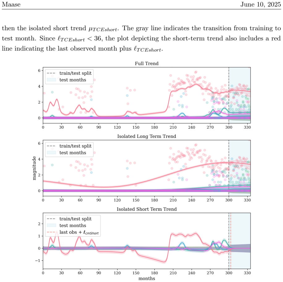
The load-bearing machinery is a two-stage Gaussian-process decomposition. First, a one-dimensional GP over months models each grid cell's logged fatality series as a sum of a smooth long-term function (squared-exponential kernel) and a rougher short-term function (Matérn-3/2 kernel); the same two-kernel structure is then fit to the spatial exposure surface, with the spatial field itself estimated by a two-dimensional GP that lets conflict magnitude radiate into neighboring cells. The kernel lengthscales, estimated by maximum a posteriori, control how far past violence informs the future: the long temporal lengthscale of about 122 months reaches across the full 36-month test window, while the short lengthscale of about 4 months decays quickly. From the extrapolated mean functions the paper derives level, slope, acceleration, and cumulative sums, yielding 24 candidate features; forward selection keeps four, and a random-forest ensemble converts them into forecast probabilities.
What would settle it
The assumption fails if the February 2015 counteroffensive in northeastern Nigeria is not an isolated case: one could test a full set of out-of-sample forecast months against observed conflict onsets after sudden reversals, measuring whether prediction error spikes in the months after any rapid regional escalation or de-escalation. A cleaner test would evaluate the same GP features on a later period the benchmark never used, such as 2018-2020, and check whether the AP/AUC margin against the full benchmark widens or collapses as the stationarity window ages.
Extended reading notes
Core claim
The paper's central claim is that the latent temporal and spatial patterns of conflict can be modeled as smooth functions and extrapolated: a Gaussian process with a squared-exponential kernel for a long-term trend and a Matérn-3/2 kernel for a short-term trend, applied first to each cell's conflict timeline and then to the spatial field of exposure, yields features that carry nearly all the predictive signal available in past violence. Estimated lengthscales, about 4 months for the short temporal trend, 122 months for the long temporal trend, and roughly one grid cell for spatial diffusion, are learned from data rather than fixed by the researcher. On the benchmark's 36-month out-of-sample test, the four GP-derived features reach AP = 0.2704 and AUC = 0.9318. The paper stresses that the result is not a rival full early-warning system but a component that estimates conflict exposure and could be incorporated into larger systems.
Load-bearing premise
The claim stands on the assumption that the way conflict spreads through time and space is stable enough for patterns learned from 1990-2014 data to describe 2015-2017, so the estimated lengthscales stay meaningful when the Gaussian-process functions are extrapolated forward.
Editorial extensions
If this is right
- Four GP-derived features from past conflict patterns alone can match or beat the conflict-history component of a full early-warning system on 36-month forecasts.
- The extrapolation is done in one shot without a sliding window or one-step-ahead refitting, so no data is lost to leads or lags and the design stays out-of-sample.
- Estimated lengthscales give a heuristic forecast horizon: signal from a trend reaches roughly one lengthscale beyond the last observed month, after which uncertainty dominates.
- The same features can serve as control variables for conflict traps and spatial diffusion in causal or parametric studies, not just as forecast inputs.
- The approach naturally extends to regression targets, such as forecasting conflict magnitude, because the GP estimates a continuous function of logged fatalities.
Reading between the lines
- The February 2015 failure suggests a natural extension: pair the GP exposure features with a regime-change or early-onset detector, so the lengthscale structure describes baseline exposure while a separate module flags abrupt breaks in conflict dynamics.
- The estimated lengthscales could be compared across regions, conflict types, or time periods as descriptive quantities, effectively turning a forecasting device into a measurement instrument for how long conflict traps last and how far diffusion reaches.
- A stress test worth running is the same pipeline on other continents or on non-state conflict data; if the parsimony result persists, the dominance of past-conflict signal in early warning is general rather than specific to Africa.
- Because the GP features are continuous and come with uncertainty estimates, they could support decision-theoretic early warning, flagging cells where predicted exposure is high and uncertain, rather than only a binary conflict probability.
Editorial analysis
A structured set of objections, weighed in public.
Referee Report
Summary. The paper proposes a two-stage Gaussian-process approach for estimating and extrapolating temporal and tempo-spatial conflict exposure from monthly PRIO-grid conflict data. From the estimated GP trends the author derives 24 features (levels, slopes, accelerations, cumulative sums for full, short-term, and long-term components), selects four via forward feature selection, and feeds them into a random-forest ensemble to forecast binary conflict onset in Africa. The model is evaluated on the same 36-month out-of-sample test period used by ViEWS (2015–2017), reporting AP = 0.2704 and AUC = 0.9318. The author claims this outperforms ViEWS' conflict-history component and nearly matches ViEWS' best ensemble, with an AP gap of 0.007 and an AUC gap of 0.0166. The out-of-sample discipline is mostly sound: GP features are extrapolated from training-period data only, and the random forest is scored on months not used for fitting.
Significance. If the results hold, the paper offers a parsimonious, data-driven alternative to hand-specified conflict-decay functions, with the additional benefit of uncertainty estimates and lengthscale-based heuristics for forecast horizons. The author supplies code for replication and follows ViEWS' data, units, and temporal splits in most respects, which are real strengths. However, the headline comparative claims currently lack uncertainty quantification, and one supporting comparison is based on data that the author states could not be obtained. The significance is therefore conditional on a revision that substantiates the comparison and clarifies the limits imposed by nonstationary conflict dynamics.
major comments (4)
- [Section 6.2, Table 5] The claim that the proposed approach 'only marginally' trails ViEWS' best ensemble rests on point estimates (AP 0.270 vs 0.277, AUC 0.9318 vs 0.9484) without confidence intervals, bootstrap, or seed-sensitivity analysis. On sparse monthly grid-cell data, an AP gap of 0.007 is well within plausible sampling variation, so the headline comparison is not yet established. The revision should supply uncertainty intervals for the proposed model (e.g., bootstrap over cells or months, and across random-forest seeds) and, where possible, for the ViEWS results taken from Hegre et al. (2019).
- [Section 6.2 and Figure 5] The text asserts that the approach outperforms ViEWS' best ensemble during the first three months of the forecast, but the caption of Figure 5 states that the corresponding ViEWS data could not be obtained. This claim is therefore not supported by the evidence presented. Either obtain and plot the ViEWS month-wise results, or remove or qualify the claim to what the available data actually show.
- [Section 5.1] The paper does not state explicitly whether the forward feature selection on the 24 GP-derived features was performed using only the 2012–2014 validation data or using the full 1990–2014 training set before evaluation on the 2015–2017 test period. If the test set influenced feature selection, the out-of-sample comparison would be compromised. Please clarify the selection protocol and confirm that it was nested within the training/validation split.
- [Sections 4.1 and 6.3] The GP exposure features are extrapolated under a stationarity assumption encoded in lengthscales learned from 1990–2014 (e.g., ℓ_TCE_long = 122.38 months), and Section 6.3's February 2015 Boko Haram counteroffensive is an instructive example of a rapid regime shift producing false negatives. While this does not invalidate the measured test-set scores, it limits the generalizability of the 36-month forecast claim and the interpretation of the lengthscale as a reliable forecast horizon. The revision should explicitly discuss this limitation and ideally provide a robustness check, such as evaluating shorter forecast horizons or applying a simple regime-break diagnostic, to show how performance varies under nonstationarity.
minor comments (4)
- [Abstract and throughout] There are several typographical and grammatical errors, including 'stat-of-the-art', 'phenomenons', 'For comparability,y', 'Do to the rarity', and 'asses' for 'assess'. A careful proofreading pass is needed.
- [Section 4.2] The text says that the spatial GP hyperparameters are estimated using all months in the training set, but the spatial GP is described as being estimated per month; please clarify whether the lengthscale is pooled across monthly snapshots or obtained by another aggregation procedure.
- [Figure 5] The persistence baseline is described only in the caption; the main text should define it and report its AP/AUC values so that the reader can interpret the comparison.
- [Section 8] The replication section points to a .zip file and a GitHub page but does not specify software versions, dependencies, or a random seed for the random-forest ensemble; please add an environment specification to make the code fully reproducible.
Circularity Check
No significant circularity: the forecast pipeline is genuinely out-of-sample and the ViEWS comparison is an external benchmark, not an input to the model.
full rationale
The derivation chain is self-contained with respect to the target quantity. The Gaussian process hyperparameters are estimated from conflict-magnitude data in the training period (Sections 4.1 and 4.2, Tables 1–3), and the GP functions are extrapolated into the 2015–2017 test months using only pre-2015 data, as stated: 'I do not use any data on conflict magnitude from the test set to do this – only data from the train set, the hyperparameters estimated, and the specifications presented above.' The random forest is then trained on the training/validation periods and evaluated on the held-out 36-month test set, so the headline AP = 0.2704 and AUC = 0.9318 are true out-of-sample scores. The comparison to ViEWS uses reported results from Hegre et al. (2019), an external published benchmark; the paper does not fit any parameter to those ViEWS numbers, and the claim of outperforming the conflict-history component is a comparison of independently evaluated models, not a tautology. The only self-citation in the paper is the author's own dissertation in the author's note and reference list, which is provenance material and is not load-bearing for any technical claim. Using the validation set to choose GP specifications and the four RF features is standard model selection, and the final evaluation is still on an untouched test period. No equation defines the predicted conflict target in terms of the fitted GP values, and no fitted parameter is renamed as a prediction. Any concerns about nonstationarity, uncertainty intervals, or the difficulty of obtaining month-wise ViEWS data are validity limitations, not circularity.
Assumptions & free parameters
free parameters (15)
- ℓ_TCE_short =
4.09
- η_TCE_short =
0.32
- ℓ_TCE_long =
122.38
- η_TCE_long =
0.50
- ε_TCE =
0.8
- ℓ_SCE =
0.72
- η_SCE =
0.027
- ε_SCE =
0.11
- ℓ_TSCE_short =
7.17
- η_TSCE_short =
0.04
- ℓ_TSCE_long =
74.72
- η_TSCE_long =
0.08
- ε_TSCE =
0.06
- Conflict timeline inclusion threshold =
at least 8 months of conflict in one year
- Spatial subset size =
top 60 cells per month
assumptions (8)
- domain assumption The latent conflict process is smooth and can be approximated by additive squared-exponential and Matern-3/2 functions.
- domain assumption The covariance structure and hyperparameters estimated on 1990-2014 data remain valid for the 2015-2017 test period.
- ad hoc to paper Timelines with little or no conflict can be excluded from hyperparameter estimation, and the resulting global hyperparameters still apply to all cells.
- ad hoc to paper The per-month spatial GP and subsequent temporal GP can be estimated in two stages without jointly modeling space-time interactions.
- ad hoc to paper Slightly informative priors on the lengthscales suffice to separate long-term and short-term trends.
- domain assumption A zero mean function m0 is adequate for the extrapolation horizons used here.
- domain assumption UCDP bestsb fatality estimates are a reliable measure of conflict existence and intensity.
- domain assumption The validation set is representative of the test set for model selection.
Cite this review
Pith. "Pith review of The Currents of Conflict: Decomposing Conflict Trends with Gaussian Processes." pith.science (2026). https://pith.science/paper/4PLZ2FPO
@misc{pith2026250606828,
  author       = {Pith},
  title        = {Pith review of: The Currents of Conflict: Decomposing Conflict Trends with Gaussian Processes},
  year         = {2026},
  howpublished = {\url{https://pith.science/paper/4PLZ2FPO}},
  note         = {Machine review of arXiv:2506.06828}
}
read the original abstract
I present a novel approach to estimating the temporal and spatial patterns of violent conflict. I show how we can use highly temporally and spatially disaggregated data on conflict events in tandem with Gaussian processes to estimate temporospatial conflict trends. These trends can be studied to gain insight into conflict traps, diffusion and tempo-spatial conflict exposure in general; they can also be used to control for such phenomenons given other estimation tasks; lastly, the approach allow us to extrapolate the estimated tempo-spatial conflict patterns into future temporal units, thus facilitating powerful, stat-of-the-art, conflict forecasts. Importantly, these results are achieved via a relatively parsimonious framework using only one data source: past conflict patterns.
Figures


Figures from the paper (3 more)


Reference graph
Works this paper leans on
-
[1]
Bara, C. (2018). Legacies of violence: Conflict-specific capital and the postconflict diffusion of civil war. Journal of Conflict Resolution , 62(9):1991--2016
2018
-
[2]
and Rupert, M
Bayer, R. and Rupert, M. C. (2004). Effects of civil wars on international trade, 1950-92. Journal of Peace Research , 41(6):699--713
2004
-
[3]
N., and Tucker, R
Beck, N., Katz, J. N., and Tucker, R. (1998). Taking time seriously: Time-series-cross-section analysis with a binary dependent variable. American Journal of Political Science , 42(4):1260--1288
1998
-
[4]
Boyd, K., Eng, K. H., and Page, C. D. (2013). Area under the precision-recall curve: point estimates and confidence intervals. In Joint European conference on machine learning and knowledge discovery in databases , pages 451--466. Springer
work page 2013
-
[5]
Buhaug, H. and Gleditsch, K. S. (2008). Contagion or confusion? why conflicts cluster in space. International Studies Quarterly , 52(2):215--233
work page 2008
-
[6]
Cederman, L.-E., Gleditsch, K. S., and Buhaug, H. (2013). Inequality, grievances, and civil war . Cambridge University Press
work page 2013
-
[7]
Cederman, L.-E., Gleditsch, K. S., and Wucherpfennig, J. (2017). Predicting the decline of ethnic civil war: Was gurr right and for the right reasons? Journal of Peace Research , 54(2):262--274
work page 2017
-
[8]
Cederman, L.-E. and Weidmann, N. B. (2017). Predicting armed conflict: Time to adjust our expectations? Science , 355(6324):474--476
work page 2017
Show all 48 references
-
[9]
Chadefaux, T. (2017). Conflict forecasting and its limits. Data Science , 1(1-2):7--17
2017
-
[10]
Collier, P. (1999). On the economic consequences of civil war. Oxford economic papers , 51(1):168--183
1999
-
[11]
and Hoeffler, A
Collier, P. and Hoeffler, A. (2004). Greed and grievance in civil war. Oxford Economic Papers , 56(4):563--595
2004
-
[12]
Corones, M. (2015). Central african republic profile - timeline. Accessed 10-05-2021
2015
-
[13]
and Felter, J
Crost, B. and Felter, J. (2015). Is conflict contagious? evidence from a natural experiment. Technical report, Households in Conflict Network, The University of Sussex
2015
-
[14]
Fearon, J. D. and Laitin, D. D. (2003). Ethnicity, insurgency, and civil war. American Political Science Review , 97(1):75–90
2003
-
[15]
Friedman, J., Hastie, T., and Tibshirani, R. (2001). The elements of statistical learning . Springer series in statistics New York, NY, USA:
2001
-
[16]
Gelfand, A. E. and Schliep, E. M. (2016). Spatial statistics and gaussian processes: A beautiful marriage. Spatial Statistics , 18:86--104
2016
-
[17]
S., Carlin, J
Gelman, A., Stern, H. S., Carlin, J. B., Dunson, D. B., Vehtari, A., and Rubin, D. B. (2013). Bayesian data analysis - third edition . Chapman and Hall/CRC
2013
-
[18]
Genton, M. G. (2001). Classes of kernels for machine learning: a statistics perspective. Journal of machine learning research , 2(Dec):299--312
2001
-
[19]
A., Bates, R
Goldstone, J. A., Bates, R. H., Epstein, D. L., Gurr, T. R., Lustik, M. B., Marshall, M. G., Ulfelder, J., and Woodward, M. (2010). A global model for forecasting political instability. American Journal of Political Science , 54(1):190--208
2010
-
[20]
and Garcia, E
He, H. and Garcia, E. A. (2008). Learning from imbalanced data. IEEE Transactions on Knowledge & Data Engineering , 9:1263--1284
2008
-
[21]
Hegre, H., Allansson, M., Basedau, M., Colaresi, M., Croicu, M., Fjelde, H., Hoyles, F., Hultman, L., H \"o gbladh, S., Jansen, R., et al. (2019). Views: a political violence early-warning system. Journal of peace research , 56(2):155--174
2019
-
[22]
W., Nyg rd, H
Hegre, H., Metternich, N. W., Nyg rd, H. M., and Wucherpfennig, J. (2017a). Introduction: Forecasting in peace research
2017
-
[23]
M., and Landsverk, P
Hegre, H., Nyg rd, H. M., and Landsverk, P. (2021). Can we predict armed conflict? how the first 9 years of published forecasts stand up to reality. International Studies Quarterly
2021
-
[24]
M., and R der, R
Hegre, H., Nyg rd, H. M., and R der, R. F. (2017b). Evaluating the scope and intensity of the conflict trap: A dynamic simulation approach. Journal of Peace Research , 54(2):243--261
2017
-
[25]
and Sambanis, N
Hegre, H. and Sambanis, N. (2006). Sensitivity analysis of empirical results on civil war onset. Journal of Conflict Resolution , 50(4):508--535
2006
-
[26]
N., and M rup, M
Herlau, T., Schmidt, M. N., and M rup, M. (2016). Introduction to machine learning and data mining. Lecture notes of the course of the same name given at DTU (Technical University of Denmark)
2016
-
[27]
and Weinstein, J
Humphreys, M. and Weinstein, J. M. (2007). Demobilization and reintegration. Journal of conflict resolution , 51(4):531--567
2007
-
[28]
Lock, P. (1997). Armed conflicts and small arms proliferation: Refocusing the research agenda. Policy Sciences , 30(3):117--132
1997
-
[29]
D., Weingarten Jr, J
Mason, T. D., Weingarten Jr, J. P., and Fett, P. J. (1999). Win, lose, or draw: Predicting the outcome of civil wars. Political Research Quarterly , 52(2):239--268
1999
-
[30]
McElreath, R. (2018). Statistical Rethinking: A Bayesian Course with Examples in R and Stan . CRC Press
2018
-
[31]
and Ramos, F
Melkumyan, A. and Ramos, F. (2011). Multi-kernel gaussian processes. In Twenty-second international joint conference on artificial intelligence . Citeseer
2011
-
[32]
and McBratney, A
Minasny, B. and McBratney, A. B. (2005). The mat \'e rn function as a general model for soil variograms. Geoderma , 128(3-4):192--207
2005
-
[33]
D., and Linke, A
O'Loughlin, J., Witmer, F. D., and Linke, A. M. (2010). The afghanistan-pakistan wars, 2008-2009: Micro-geographies, conflict diffusion, and clusters of violence. Eurasian Geography and Economics , 51(4):437--471
2010
-
[34]
Perry, C. (2013). Machine learning and conflict prediction: a use case. Stability: International Journal of Security & Development , 56(2(3))
2013
-
[35]
Schrodt, P. A. (2014). Seven deadly sins of contemporary quantitative political analysis. Journal of Peace Research , 51(2):287--300
2014
-
[36]
and Weidmann, N
Schutte, S. and Weidmann, N. B. (2011). Diffusion patterns of violence in civil wars. Political Geography , 30(3):143--152
2011
-
[37]
Singer, J. D. (1973). The peace researcher and foreign policy prediction. Peace Science Society (International) , 21:1--13
1973
-
[38]
Slantchev, B. L. (2012). Borrowed power: Debt finance and the resort to arms. American Political Science Review , pages 787--809
2012
-
[39]
Stedman, S. J. (1997). Spoiler problems in peace processes. International security , 22(2):5--53
1997
-
[40]
Su, W., Yuan, Y., and Zhu, M. (2015). A relationship between the average precision and the area under the roc curve. In Proceedings of the 2015 International Conference on The Theory of Information Retrieval , pages 349--352. ACM
2015
-
[41]
Toft, M. D. (2010). Ending civil wars: a case for rebel victory? International Security , 34(4):7--36
2010
-
[42]
F., Strand, H., and Buhaug, H
Tollefsen, A. F., Strand, H., and Buhaug, H. (2012). Prio-grid: A unified spatial data structure. Journal of Peace Research , 49(2):363--374
2012
-
[43]
von der Maase, S. P. (2023). A Lens to Learn Through: Conflict Studies in the Age of Computational Methods . Ph.d. dissertation, University of Copenhagen, Department of Political Science and the Center for Social Data Science (SODAS). Supervised by Lene Hansen and Jacob Gerner...
2023
-
[44]
Ward, M. D. and Beger, A. (2017). Lessons from near real-time forecasting of irregular leadership changes. Journal of Peace Research , 54(2):141--156
2017
-
[45]
D., Greenhill, B
Ward, M. D., Greenhill, B. D., and Bakke, K. M. (2010). The perils of policy by p-value: Predicting civil conflicts. Journal of Peace Research , 47(4):363--375
2010
-
[46]
Weidmann, N. B. and Ward, M. D. (2010). Predicting conflict in space and time. Journal of Conflict Resolution , 54(6):883--901
2010
-
[47]
Williams, C. K. and Rasmussen, C. E. (2006). Gaussian processes for machine learning , volume 2. MIT Press Cambridge, MA
2006
-
[48]
Wood, E. J. (2008). The social processes of civil war: The wartime transformation of social networks. Annu. Rev. Polit. Sci. , 11:539--561
2008
Reviewed August 7, 2026 · model on record in the stance chip above.
Discussion (0). Sign in to comment.