Graph-Based Physics-Guided Urban PM2.5 Air Quality Imputation with Constrained Monitoring Data

Dong Yoon Lee; Hui Wei; Shangjie Du; Shijia Pan; Zhizhang Hu

REVIEW 4 major objections 4 minor 82 references

Graph-Based Physics-Guided Urban PM2.5 Air Quality Imputation with Constrained Monitoring Data

T0 review · 4 major / 4 minor · reviewed 2026-08-07 · deepseek-v4-flash

Challenge this review Re-run · record.json Download PDF Read on arXiv ↗

Pith's one-line read A physics-guided graph neural network cuts PM2.5 imputation error by up to 56% on sparse urban monitor networks.

desk verdict Plausible physics-guided GNN for PM2.5 imputation that is honest about its limits, but the headline result rests on a single sensor split and no ablations. read the letter →

arxiv 2506.06917 v1 pith:JFMQPCWM submitted 2025-06-07 cs.LG cs.AI

Shangjie Du , Hui Wei , Dong Yoon Lee , Zhizhang Hu , Shijia Pan This is my paper

classification cs.LGcs.AI

keywords PM2.5imputationgraphneuralnetworksphysics-guidedlearningsparsemonitoringconvection-diffusionequationspatialinterpolationurbanairqualitywind-basededgefeatures

verification ladder T0 review T1 audit T2 compute T3 formal

The pith

A machine-rendered reading of the paper's core claim, the machinery that carries it, and where it could break.

The reading

GraPhy is a graph neural network that predicts PM2.5 at unmonitored locations from sparse sensor readings plus city-level wind data, and this paper claims it outperforms six interpolation and learning baselines on real data from California's San Joaquin Valley. The design maps the convection-diffusion equation onto three network modules—diffusion, convection, and local sources/sinks—so that coarse wind information is encoded as pairwise edge features rather than requiring fine-grained meteorology at every station. Across held-out sensors, the paper reports 24–56% lower mean squared error, 22–51% lower mean absolute error, and 9–50% higher R-squared than the baselines, with consistent advantages across spatial heterogeneity levels. The motivation is that monitoring-constrained, often disadvantaged regions lack the dense networks needed by standard interpolation methods, so better imputation from limited data would improve exposure estimates and public-health analysis.

What carries the argument

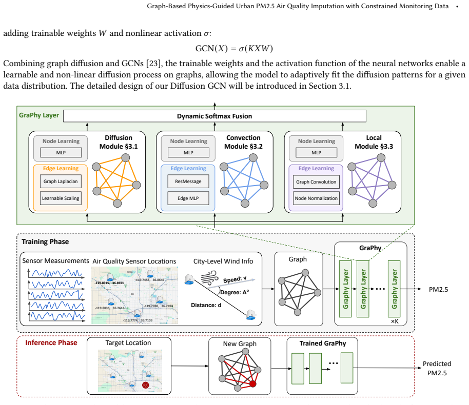
The load-bearing mechanism is the convection-diffusion equation $\partial x/\partial t = d\,\nabla^2 x - v\cdot\nabla x + R(s,t)$, discretised onto a sensor graph. Diffusion becomes a normalized graph Laplacian scaled by a learnable vector; convection becomes residual message passing over wind-based edge features (speed, directional similarity, distance); local sources become a graph convolution with degree normalization. A dynamic softmax fusion combines the three modules' features into each layer's output, and masked-sensor training with a dummy node at inference lets the same graph machinery handle unmonitored locations.

What would settle it

Re-run the same experiment on multiple random 28/4/9 splits (for example, ten partitions) and compare the distribution of MSE and MAE; if GraPhy does not beat inverse distance weighting and ordinary kriging in most splits, the reported 24–56% improvement is an artifact of the single chosen test set.

Watch

Extended reading notes

Core claim

The central claim is that a GNN whose layers mirror the three terms of the convection-diffusion equation can interpolate PM2.5 accurately using only sparse measurements and one city-level wind reading. The Diffusion module applies a graph Laplacian with a learnable vector as the diffusion coefficient; the Convection module builds edge features from wind speed, the cosine similarity between wind direction and the sensor-pair direction, and distance; the Local module uses graph convolution with degree normalization to capture local sources and sinks. A dynamic softmax fusion weights the three module outputs per input. The model is trained by masking one sensor and recovering it, then applied to a new graph that adds the unmonitored location as a dummy node. The paper reports that this architecture outperforms all tested baselines and, unlike a prior physics-guided GNN variant requiring per-station wind data, works when only city-level wind is available.

Load-bearing premise

The strongest load-bearing assumption is that the single random split into 28 training, 4 validation, and 9 test sensors yields a test set representative enough of the whole network that the reported error reductions generalize; a different split could change or reverse the ranking.

Editorial extensions

If this is right

If the results hold, sparse citizen-science sensor networks can produce higher-resolution PM2.5 maps without adding monitors or per-station weather stations.
The three-module decomposition offers a template for other sensor-imputation problems: align network modules with the terms of the governing transport equation and encode the coarsest available meteorology as edge features.
The reported gains are largest in the low-to-moderate PM2.5 range that dominates the test data; for high-pollution events above roughly 80 µg/m³, baseline models perform comparably.
The superiority is bounded by sensor density: at densities below about 0.16 sensors per square mile, simpler methods such as inverse distance weighting and Gaussian-process interpolation match or beat GraPhy.
Graph-based models including GraPhy degrade sharply at the lowest density tested, so the architecture is suited to moderately sparse networks rather than extremely sparse ones.

Reading between the lines

Editorial extensions of the paper, not claims the author makes directly.

Repeated cross-validation over sensor splits is the most direct check on whether the reported margins hold beyond one test set; the paper's single split leaves this open.
The dynamic softmax weights could be analyzed per time step to identify when the model attributes predictions to convection versus local sources, turning the fusion module into an interpretability probe for pollution episodes.
The same edge-feature recipe—wind speed, directional cosine, distance—should transfer to other transported environmental quantities such as ozone or urban heat when only city-scale weather is available.
A density-aware mixture that weights GraPhy against inverse distance weighting or kriging as local sensor density falls could extend the usable range, since each method dominates in a different density regime.

Share X Bluesky LinkedIn Reddit HN

Editorial analysis

A structured set of objections, weighed in public.

Desk editor's note, referee report, and a circularity audit.

Desk Editor's Note

read the letter

First, the honest version: this is a competent engineering extension of the authors' own BuildSys 2024 GraPhy paper, adapted to city-level (single-station) wind data. The new pieces—wind-based edge features, per-feature learnable diffusion scaling, residual message passing, and dynamic softmax fusion—are reasonable and clearly motivated for monitoring-constrained regions. The evaluation on real Fresno data includes sensible baselines (classical kriging/IDW, GNN, LSTM) and an informative sensor-density robustness study. The paper is unusually candid in Section 6: it admits the model stops being best at low sensor densities and that it uses a single data source. I read Section 6 as a genuine limitation statement, not a formality.

The soft spots are real, though. The headline 9–56% improvement and the 'consistently outperforms' claim rest on one random split of 41 sensors into 28/4/9, with no repeated splits or cross-validation. Nine test sensors are too few to establish a stable ranking, and the paired t-test (p<0.0001) is applied to 26,352 hourly test estimates that are heavily autocorrelated—so it doesn't answer the split-selection question. The density experiment shows exactly why this matters: at 0.11/mi2 and 0.06/mi2, GraPhy no longer wins, so the advantage is regime-dependent. The abstract overstates. There is also no ablation of the three modules or the fusion, so we can't attribute the gain to any specific design decision.

What is not a problem: the physics is used as architectural inspiration; the learnable diffusion coefficient is fitted, not derived from first principles, and the paper doesn't pretend otherwise. The self-citation is legitimate since this is an extension of their own published work, though the BuildSys paper isn't in the reference list, which should be fixed.

Overall: this is a solid workshop-to-short-paper contribution, arguably a solid conference paper if the evaluation were hardened. It deserves serious peer review, but a referee should ask for repeated splits (or at least a bootstrap over sensors), ablations, and preferably code/data release. I'd frame the abstract's 'consistently outperforms' down to 'achieves best average performance on this split, with known degradation at low density.'

Referee Report

4 major / 4 minor

Summary. The paper proposes GraPhy, a graph neural network that integrates three physics-inspired modules (diffusion, convection, local source/sink) and a dynamic softmax fusion layer for spatial imputation of PM2.5 from sparse monitoring networks. Using four months of hourly calibrated citizen-science data from 41 sensors in Fresno, California, and city-level wind data, the authors train the model by masking one sensor at a time and evaluate it on nine held-out sensors. They report that GraPhy achieves the best MSE, MAE, and R2 among six baselines, with 24%–56% MSE reduction, and that it outperforms baselines across PM2.5 concentration bins and spatial heterogeneity bins. They also analyze robustness to sensor density and model size.

Significance. GraPhy is a reasonable engineering contribution: it adapts a physics-inspired GNN to coarse city-level wind data, uses a learnable per-feature diffusion scaling, and is evaluated on a real, under-served region rather than synthetic data. The paper is transparent about limitations (e.g., Section 4.5.4 and Section 6). If the performance claims were supported by proper statistical evidence and ablations, the work would be useful for environmental monitoring applications. The real-world dataset, the city-level wind edge features, and the comparison with an AirPhyNet variant adapted to interpolation are all positive aspects. However, the current evidence does not establish that GraPhy 'consistently outperforms' baselines, because the evaluation uses a single sensor split and an invalid significance test, and no ablation isolates the contribution of the physics-guided modules. These gaps are fixable within the manuscript's scope.

major comments (4)

[Section 4.2 and Section 4.5.1] The headline comparison rests on a single 28/4/9 sensor split (Section 4.2). Because the nine test sensors are spatially correlated, the reported 24%–56% MSE reduction and the 'consistently outperforms' claim may be an artifact of which sensors were held out. The five-seed repetition in Section 4.5 averages over initialization and training-sample permutation only; it does not sample the test-sensor distribution. I request repeated spatial splits (e.g., leave-sensor-out or k-fold over the 41 sensors) with per-split metrics and report mean and standard deviation or confidence intervals, or otherwise demonstrate that the ranking is stable across test-sensor subsets.
[Section 4.5.1] Applying a paired t-test to 26,352 hourly test estimates is not a valid significance test: hourly PM2.5 observations are strongly autocorrelated in time, and the nine test sensors provide clustered rather than independent samples. The p<0.0001 result therefore does not establish that GraPhy is significantly better than the baselines. Use a block bootstrap over hourly sequences or a paired test at the sensor-split level (e.g., Wilcoxon over per-split metrics) to support inferential statements.
[Section 3 and Section 4.5] The paper attributes GraPhy's gains to the physics-guided design (diffusion, convection, local modules, and dynamic fusion), but no ablation isolates these components. Without ablating or replacing each module (e.g., removing the physics modules, replacing dynamic fusion with fixed weights, or removing residual message passing), the experiments cannot distinguish the contribution of the physics-guided design from generic GNN capacity. This is load-bearing for the claim that 'the effectiveness of our model design' is demonstrated.
[Section 4.5.4 and Table 2] GraPhy is not the best model at sensor densities 0.11/mi2 and 0.06/mi2, where IDW and GP outperform it. This contradicts the broad framing that GraPhy is designed for 'monitoring-constrained regions'; the claims in the abstract and conclusion should be qualified to the evaluated density range (at least 0.16/mi2), or the model should be adapted with a density-aware mechanism. The Discussion (Section 6) acknowledges a future mixture model, which is appropriate, but the current text overstates robustness.

minor comments (4)

[Section 4.5.1] The phrase '24%–56% reduce on MSE' should be '24%–56% reduction in MSE'; the same wording issue appears in the caption of Figure 8.
[Section 4.5.2 and Figure 10] The ratio plots in Figures 10 and 12 would be more informative with sample counts or confidence intervals per bin, since the high-PM2.5 and high-heterogeneity bins contain very few samples.
[Section 3.2] The description of the wind-direction similarity w_A is verbal only; an explicit formula would clarify how the cosine of the angle between wind direction and sensor-pair direction is computed.
[Section 4.1] Please state explicitly how the 41 sensors used here compare with the 51 originally collected, and whether the data and code will be released; this would support reproducibility.

Circularity Check

0 steps flagged · score 0.0 of 10

No significant circularity: GraPhy's performance claim rests on held-out sensor evaluation, and the physics equation is used only as architectural inspiration.

full rationale

No circularity is present in the paper's derivation or evaluation chain. The central claim, that GraPhy outperforms baselines on PM2.5 imputation, is supported by experiments on test sensors excluded from training (Section 4.2: 28 training, 4 validation, 9 test sensors), so the reported predictions are not equivalent to the model's training inputs by construction. The convection-diffusion equation (Eq. 2) is used as design motivation for the Diffusion, Convection, and Local modules, not as a source of constants that are then reported as predictions; the learnable diffusion coefficient is an architectural parameter fitted to data, and the paper does not present it as a measured or predicted physical quantity. The spatial-heterogeneity metric (Eq. 3) is an analysis tool, not an output derived from the model. The BuildSys extension footnote is a self-citation but is only a provenance statement and is not load-bearing for any result. The absence of repeated sensor splits is an experimental robustness concern, not a circularity concern. The evaluation is self-contained and externally benchmarked, so no fitted input is renamed as a prediction and no self-citation chain forces the outcome.

Assumptions & free parameters 3 free parameters · 4 assumptions · 0 invented entities

The paper's central claim is an empirical model comparison, so the main free parameters are the neural network weights and hyperparameters. The 'physics-guided' aspect is architectural inspiration rather than a constraint: the diffusion coefficient is a learnable vector rather than a physical constant, and the model is trained end-to-end on data. No new physical entities are introduced.

free parameters (3)

Diffusion coefficient vector l (per-feature learnable scaling) = learned from data
Section 3.1: replaces fixed scalar diffusion coefficient with a learnable vector of the same dimension as output features; fitted by gradient descent, not derived from physical constraints.
All MLP/GCN weights (node, edge, message, update, fusion) = trained with Adam, lr 0.0001
Standard supervised training; the model's predictive power comes from these fitted parameters, so they are free parameters of the method.
Architecture hyperparameters (layers, hidden dimension, batch size) = 5 layers, 512 hidden, batch 32
Chosen by the authors; only model size ablations are reported, no full sensitivity analysis for these values.

assumptions (4)

domain assumption The convection-diffusion equation (Section 2.2) adequately describes the relevant PM2.5 dynamics at urban street scale.
The three modules are designed to mimic the PDE's three terms; the equation omits chemical reactions, deposition, and source timing and is not used as a hard constraint.
domain assumption A single city-level wind station provides sufficient wind information for all sensor pairs.
Section 3.2 and Table 1: one wind station for all of Fresno; if wind varies spatially, the cosine similarity edge features are mis-specified.
domain assumption Mask-and-recover training with one masked sensor is a faithful proxy for predicting at truly unmonitored locations.
The dummy node during training is a sensor whose true value is masked; the model never trains on locations that are absent from the sensor network, so the dummy node distribution may differ at inference.
standard math Standard backpropagation and GNN message-passing machinery work as assumed.
No formal verification; relies on standard deep learning background.

how reviews work

0 comments

Cite this review

Pith. "Pith review of Graph-Based Physics-Guided Urban PM2.5 Air Quality Imputation with Constrained Monitoring Data." pith.science (2026). https://pith.science/paper/JFMQPCWM

@misc{pith2026250606917,
  author       = {Pith},
  title        = {Pith review of: Graph-Based Physics-Guided Urban PM2.5 Air Quality Imputation with Constrained Monitoring Data},
  year         = {2026},
  howpublished = {\url{https://pith.science/paper/JFMQPCWM}},
  note         = {Machine review of arXiv:2506.06917}
}

read the original abstract

This work introduces GraPhy, a graph-based, physics-guided learning framework for high-resolution and accurate air quality modeling in urban areas with limited monitoring data. Fine-grained air quality monitoring information is essential for reducing public exposure to pollutants. However, monitoring networks are often sparse in socioeconomically disadvantaged regions, limiting the accuracy and resolution of air quality modeling. To address this, we propose a physics-guided graph neural network architecture called GraPhy with layers and edge features designed specifically for low-resolution monitoring data. Experiments using data from California's socioeconomically disadvantaged San Joaquin Valley show that GraPhy achieves the overall best performance evaluated by mean squared error (MSE), mean absolute error (MAE), and R-square value (R2), improving the performance by 9%-56% compared to various baseline models. Moreover, GraPhy consistently outperforms baselines across different spatial heterogeneity levels, demonstrating the effectiveness of our model design.

Figures

Figures reproduced from arXiv: 2506.06917 by the authors.

**Figure 1.** San Joaquin Valley (SJV)’ challenges regarding air pollutant exposure: (a) The basin terrain of the SJV traps air pollutants easily; (b) [PITH_FULL_IMAGE:figures/full_fig_p002_1.png] view at source ↗

**Figure 2.** Purple Air sensor network deployment in Santa Clara and Fresno. (a) Santa Clara has a 10 [PITH_FULL_IMAGE:figures/full_fig_p002_2.png] view at source ↗

**Figure 3.** Examples of high and low spatial heterogeneity (SH), where each point represents the PM2.5 concentration at a sensing location. [PITH_FULL_IMAGE:figures/full_fig_p003_3.png] view at source ↗

Figures from the paper (8 more)

**Figure 4.** Figure 4: GraPhy Overview. The model inputs sparse air quality sensor measurements, sensor location, and city-level wind information. These measurements determine the graph’s node and edge features. A GNN model consisting of multiple GraPhy layers is used to model the air qualit…

**Figure 5.** Figure 5: Diffusion Module 𝜙 [PITH_FULL_IMAGE:figures/full_fig_p007_5.png]

**Figure 8.** Figure 8: Prediction Accuracy of All Models on the Test Set. [PITH_FULL_IMAGE:figures/full_fig_p009_8.png]

**Figure 9.** Figure 9: Distribution of Ground-Truth PM2.5 Values and MAE Performance of [PITH_FULL_IMAGE:figures/full_fig_p011_9.png]

**Figure 10.** Figure 10: Ratio of the MAE from the baseline models to that of the [PITH_FULL_IMAGE:figures/full_fig_p012_10.png]

**Figure 11.** Figure 11: Distribution of Spatial Heterogeneity values and MAE Performance of [PITH_FULL_IMAGE:figures/full_fig_p012_11.png]

**Figure 12.** Figure 12: Ratio of the MAE from the baseline models to that of the [PITH_FULL_IMAGE:figures/full_fig_p013_12.png]

**Figure 13.** Figure 13: Performance Across Different Model Sizes. The left y-axis represents model size ( [PITH_FULL_IMAGE:figures/full_fig_p015_13.png]

Discussion (0). Sign in to comment.

Reference graph

Works this paper leans on

82 extracted references · 58 canonical work pages

[1]

Environmental Protection Agency

U.S. Environmental Protection Agency. 2024. Links Between Air Pollution and Childhood Asthma. https://www.epa.gov/sciencematters/links-between-air- pollution-and-childhood-asthma Accessed: 2024-06-10

2024
[2]

Mohamed Aghzal, Erion Plaku, Gregory J Stein, and Ziyu Yao. 2025. A Survey on Large Language Models for Automated Planning.arXiv preprint arXiv:2502.12435(2025)

arXiv 2025
[3]

Purple Air. 2024. Research Considerations. https://community.purpleair.com/t/research-considerations/9144. Accessed: 2024-07-21

2024
[4]

Michael M Bronstein, Joan Bruna, Yann LeCun, Arthur Szlam, and Pierre Vandergheynst. 2017. Geometric deep learning: going beyond euclidean data.IEEE Signal Processing Magazine34, 4 (2017), 18–42

2017
[5]

Xinlei Chen, Susu Xu, Xinyu Liu, Xiangxiang Xu, Hae Young Noh, Lin Zhang, and Pei Zhang. 2020. Adaptive hybrid model-enabled sensing system (HMSS) for mobile fine-grained air pollution estimation.IEEE Transactions on Mobile Computing21, 6 (2020), 1927–1944

work page 2020
[6]

Yun Cheng, Xiucheng Li, Zhijun Li, Shouxu Jiang, Yilong Li, Ji Jia, and Xiaofan Jiang. 2014. AirCloud: A cloud-based air-quality monitoring system for everyone. InProceedings of the 12th ACM Conference on Embedded Network Sensor Systems. 251–265

work page 2014
[7]

Denise Chow. 2024. 131 Million in U.S. Live in Areas with Unhealthy Pollution Levels, Lung Association Reports. https://www.nbcnews.com/science/ environment/131-million-us-live-areas-unhealthy-pollution-levels-lung-association-rcna148795 Accessed: 2024-06-10. , Vol. 1, No. 1, Article . Publication date: September 2025. •Du and Wei et al

work page 2024
[8]

Arka Daw, Anuj Karpatne, William D Watkins, Jordan S Read, and Vipin Kumar. 2022. Physics-guided neural networks (pgnn): An application in lake temperature modeling. InKnowledge guided machine learning. Chapman and Hall/CRC, 353–372

work page 2022

Show all 82 references

[9]

Srinivas Devarakonda, Parveen Sevusu, Hongzhang Liu, Ruilin Liu, Liviu Iftode, and Badri Nath. 2013. Real-time air quality monitoring through mobile sensing in metropolitan areas. InProceedings of the 2nd ACM SIGKDD international workshop on urban computing. 1–8

2013
[10]

San Joaquin Valley Air Pollution Control District. 2021. Air Quality in San Joaquin Valley. https://ww2.valleyair.org/media/4x5ng03o/short-presentation- for-web-2021.pdf

2021
[11]

Bruce A Egan and James R Mahoney. 1972. Numerical modeling of advection and diffusion of urban area source pollutants.Journal of Applied Meteorology and Climatology11, 2 (1972), 312–322

1972
[12]

Jill A Engel-Cox, Raymond M Hoff, and ADJ Haymet. 2004. Recommendations on the use of satellite remote-sensing data for urban air quality.Journal of the Air & Waste Management Association54, 11 (2004), 1360–1371

2004
[13]

1990.User’s manual for SLAB: An atmospheric dispersion model for denser-than-air-releases

Donald L Ermak. 1990.User’s manual for SLAB: An atmospheric dispersion model for denser-than-air-releases. Technical Report. Lawrence Livermore National Lab., CA (USA)

1990
[14]

O Favez, I El Haddad, C Piot, A Boréave, E Abidi, Nicolas Marchand, J-L Jaffrezo, J-L Besombes, M-B Personnaz, J Sciare, et al. 2010. Inter-comparison of source apportionment models for the estimation of wood burning aerosols during wintertime in an Alpine city (Grenoble, Fran...

2010
[15]

Yoav Freund and Robert E Schapire. 1995. A desicion-theoretic generalization of on-line learning and an application to boosting. InEuropean conference on computational learning theory. Springer, 23–37

1995
[16]

Jerome H Friedman. 2001. Greedy function approximation: a gradient boosting machine.Annals of statistics(2001), 1189–1232

2001
[17]

Lisa Friedman and Brad Plumer. 2024. Biden Administration Announces New Pollution Standards for Power Plants.The New York Times(2024). https://www.nytimes.com/2024/04/25/climate/biden-power-plants-pollution.html Accessed: 2024-06-10

2024
[18]

Justin Gilmer, Samuel S Schoenholz, Patrick F Riley, Oriol Vinyals, and George E Dahl. 2017. Neural message passing for quantum chemistry. InInternational conference on machine learning. PMLR, 1263–1272

2017
[19]

David Gobeli, Herbert Schloesser, and Thomas Pottberg. 2008. Met one instruments BAM-1020 beta attenuation mass monitor US-EPA PM2. 5 federal equivalent method field test results. InThe Air & Waste Management Association (A&WMA) Conference, Kansas City, MO, Vol. 2. Citeseer

2008
[20]

Marco Gori, Gabriele Monfardini, and Franco Scarselli. 2005. A new model for learning in graph domains. InProceedings. 2005 IEEE international joint conference on neural networks, 2005., Vol. 2. IEEE, 729–734

2005
[21]

GridInfo. 2024. Fresno, CA Electricity Generation Summary. https://www.gridinfo.com/california/fresno

2024
[22]

Nate Gruver, Marc Finzi, Shikai Qiu, and Andrew G Wilson. 2023. Large language models are zero-shot time series forecasters.Advances in Neural Information Processing Systems36 (2023), 19622–19635

2023
[23]

Kethmi Hirushini Hettige, Jiahao Ji, Shili Xiang, Cheng Long, Gao Cong, and Jingyuan Wang. 2024. AirPhyNet: Harnessing Physics-Guided Neural Networks for Air Quality Prediction.arXiv preprint arXiv:2402.03784(2024)

2024 arXiv
[24]

Hsun-Ping Hsieh, Shou-De Lin, and Yu Zheng. 2015. Inferring air quality for station location recommendation based on urban big data. InProceedings of the 21th ACM SIGKDD international conference on knowledge discovery and data mining. 437–446

2015
[25]

Zhizhang Hu, Shangjie Du, Yuning Chen, Xuan Zhang, Wan Du, Asa Bradman, and Shijia Pan. 2023. Enhancing Fault Resilience of Air Quality Monitoring in San Joaquin Valley: A Data Equity Analysis. InProceedings of the 21st ACM Conference on Embedded Networked Sensor Systems. 514–515

2023
[26]

Zhizhang Hu, Tong Yu, Ruiyi Zhang, and Shijia Pan. 2022. CIPhy: Causal Intervention with Physical Confounder from IoT Sensor Data for Robust Occupant Information Inference. InProceedings of the 20th ACM Conference on Embedded Networked Sensor Systems. 966–972

2022
[27]

Zhizhang Hu, Yue Zhang, Ryan Rossi, Tong Yu, Sungchul Kim, and Shijia Pan. 2024. Are large language models capable of causal reasoning for sensing data analysis?. InProceedings of the Workshop on Edge and Mobile Foundation Models. 24–29

2024
[28]

Zhizhang Hu, Yue Zhang, Tong Yu, and Shijia Pan. 2022. VMA: Domain variance-and modality-aware model transfer for fine-grained occupant activity recognition. In2022 21st ACM/IEEE International Conference on Information Processing in Sensor Networks (IPSN). IEEE, 259–270

2022
[29]

Jie Huang and Kevin Chen-Chuan Chang. 2022. Towards reasoning in large language models: A survey.arXiv preprint arXiv:2212.10403(2022)

2022 arXiv
[30]

Xu Huang, Weiwen Liu, Xiaolong Chen, Xingmei Wang, Hao Wang, Defu Lian, Yasheng Wang, Ruiming Tang, and Enhong Chen. 2024. Understanding the planning of LLM agents: A survey.arXiv preprint arXiv:2402.02716(2024)

2024 arXiv
[31]

Egemen İşgüder and Özlem Durmaz İncel. 2023. FedOpenHAR: Federated Multi-Task Transfer Learning for Sensor-Based Human Activity Recognition. arXiv preprint arXiv:2311.07765(2023)

2023 arXiv
[32]

Stijn Janssen, Gerwin Dumont, Frans Fierens, and Clemens Mensink. 2008. Spatial interpolation of air pollution measurements using CORINE land cover data.Atmospheric Environment42, 20 (2008), 4884–4903

2008
[33]

Bowen Jin, Gang Liu, Chi Han, Meng Jiang, Heng Ji, and Jiawei Han. 2024. Large language models on graphs: A comprehensive survey.IEEE Transactions on Knowledge and Data Engineering(2024)

2024
[34]

Kaimaoge. 2024. IGNNK: Inductive Graph Neural Networks for Spatiotemporal Kriging. https://github.com/Kaimaoge/IGNNK

2024
[35]

Frank J Kelly and Julia C Fussell. 2015. Air pollution and public health: emerging hazards and improved understanding of risk.Environmental geochemistry and health37 (2015), 631–649

2015
[36]

Thomas N Kipf and Max Welling. 2016. Semi-supervised classification with graph convolutional networks.arXiv preprint arXiv:1609.02907(2016)

2016 arXiv
[37]

Xiao Liu, Kyongmin Yeo, and Siyuan Lu. 2022. Statistical modeling for spatio-temporal data from stochastic convection-diffusion processes.J. Amer. Statist. Assoc.117, 539 (2022), 1482–1499

2022
[38]

Yuxuan Liu, Haoyang Wang, Fanhang Man, Jingao Xu, Fan Dang, Yunhao Liu, Xiao-Ping Zhang, and Xinlei Chen. 2024. MobiAir: Unleashing Sensor Mobility for City-scale and Fine-grained Air-Quality Monitoring with AirBERT. InProceedings of the 22nd Annual International Conference on...

2024
[39]

Jun Ma, Yuexiong Ding, Jack CP Cheng, Feifeng Jiang, and Zhiwei Wan. 2019. A temporal-spatial interpolation and extrapolation method based on geographic Long Short-Term Memory neural network for PM2. 5.Journal of Cleaner Production237 (2019), 117729

2019
[40]

Randall V Martin. 2008. Satellite remote sensing of surface air quality.Atmospheric environment42, 34 (2008), 7823–7843

2008
[41]

Mostafa Mirshekari, Jonathon Fagert, Shijia Pan, Pei Zhang, and Hae Young Noh. 2020. Step-level occupant detection across different structures through footstep-induced floor vibration using model transfer.Journal of Engineering Mechanics146, 3 (2020), 04019137

2020
[42]

Tahsin Mullick, Sam Shaaban, Ana Radovic, Afsaneh Doryab, et al. 2024. Framework for ranking machine learning predictions of limited, multimodal, and longitudinal behavioral passive sensing data: combining user-agnostic and personalized modeling.JMIR AI3, 1 (2024), e47805

2024
[43]

Zeel B Patel, Palak Purohit, Harsh M Patel, Shivam Sahni, and Nipun Batra. 2022. Accurate and scalable gaussian processes for fine-grained air quality inference. InProceedings of the AAAI Conference on Artificial Intelligence, Vol. 36. 12080–12088. , Vol. 1, No. 1, Article . P...

2022
[44]

Bryan Perozzi, Bahare Fatemi, Dustin Zelle, Anton Tsitsulin, Mehran Kazemi, Rami Al-Rfou, and Jonathan Halcrow. 2024. Let your graph do the talking: Encoding structured data for llms.arXiv preprint arXiv:2402.05862(2024)

2024 arXiv
[45]

Roger A Pielke and M Uliasz. 1998. Use of meteorological models as input to regional and mesoscale air quality models—limitations and strengths. Atmospheric environment32, 8 (1998), 1455–1466

1998
[46]

Jacqueline Pinedo and Sarah Linn. 2024. Fresno is among top 10 most polluted cities in U.S., American Lung Association. Here’s why.The Fresno Bee(2024). https://www.fresnobee.com/news/local/article288061190.html

2024
[47]

PurpleAir. 2024. PurpleAir: Monitoring Air Quality. https://www2.purpleair.com/. Accessed: 2024-07-23

2024
[48]

PyTorch Geometric. 2024. PyTorch Geometric Documentation: Introduction-Minibatches. https://pytorch-geometric.readthedocs.io/en/latest/get_started/ introduction.html. Accessed: 2024-07-23

2024
[49]

Yujia Qin, Shihao Liang, Yining Ye, Kunlun Zhu, Lan Yan, Yaxi Lu, Yankai Lin, Xin Cong, Xiangru Tang, Bill Qian, et al. 2023. Toolllm: Facilitating large language models to master 16000+ real-world apis.arXiv preprint arXiv:2307.16789(2023)

2023 arXiv
[50]

Changle Qu, Sunhao Dai, Xiaochi Wei, Hengyi Cai, Shuaiqiang Wang, Dawei Yin, Jun Xu, and Ji-Rong Wen. 2025. Tool learning with large language models: A survey.Frontiers of Computer Science19, 8 (2025), 198343

2025
[51]

K Ramesh, B Rajarao, Hitesh E Chaudhari, S Angel Latha Mary, M Venkatanaresh, and Tarun Kumar Dhiman. 2024. Transfer learning approach to reduce similar IOT sensor data for industrial applications.Measurement: Sensors31 (2024), 100985

2024
[52]

Darryl Randerson. 1970. A numerical experiment in simulating the transport of sulfur dioxide through the atmosphere.Atmospheric Environment (1967)4, 6 (1970), 615–632

1967
[53]

Shubham Rohal, Dong Yoon Lee, Carlos Ruiz, Joshua Zhang, Jonathon Fagert, Jun Han, and Shijia Pan. 2024. Don’t Crosstalk to Me: Origami Structure- Augmented Sensing for Scalable Surface Pressure Monitoring. InProceedings of the 22nd ACM Conference on Embedded Networked Sensor ...

2024
[54]

Franco Scarselli, Marco Gori, Ah Chung Tsoi, Markus Hagenbuchner, and Gabriele Monfardini. 2008. The graph neural network model.IEEE transactions on neural networks20, 1 (2008), 61–80

2008
[55]

Stephen H Schneider. 1992. Introduction to climate modeling.SMR648, 6 (1992), 1677

1992
[56]

Joseph S Scire, David G Strimaitis, Robert J Yamartino, et al. 2000. A user’s guide for the CALPUFF dispersion model.Earth Tech, Inc521 (2000), 1–521

2000
[57]

Donald Shepard. 1968. A two-dimensional interpolation function for irregularly-spaced data. InProceedings of the 1968 23rd ACM national conference. 517–524

1968
[58]

CC Shir and LJ Shieh. 1974. A generalized urban air pollution model and its application to the study of SO2 distributions in the St. Louis metropolitan area. Journal of Applied Meteorology and Climatology13, 2 (1974), 185–204

1974
[59]

SJVAir. 2024. SJVAir Official Website. https://www.sjvair.com/. Accessed: 2024-07-21

2024
[60]

2011.Introduction to climate modelling

Thomas Stocker. 2011.Introduction to climate modelling. Springer Science & Business Media

2011
[61]

John M Stockie. 2011. The mathematics of atmospheric dispersion modeling.Siam Review53, 2 (2011), 349–372

2011
[62]

Terry T Um, Franz MJ Pfister, Daniel Pichler, Satoshi Endo, Muriel Lang, Sandra Hirche, Urban Fietzek, and Dana Kulić. 2017. Data augmentation of wearable sensor data for parkinson’s disease monitoring using convolutional neural networks. InProceedings of the 19th ACM internat...

2017
[63]

Department of Energy

U.S. Department of Energy. [n. d.]. Fuel economy in cold weather. https://www.fueleconomy.gov/feg/coldweather.shtml Accessed: 2024-07-22

2024
[64]

Visual Crossing. 2024. Historical Weather Data & Weather Forecast Data. https://www.visualcrossing.com/weather-data

2024
[65]

Hans Wackernagel and Hans Wackernagel. 2003. Ordinary kriging.Multivariate geostatistics: An introduction with applications(2003), 79–88

2003
[66]

Jinqiang Wang, Tao Zhu, Jingyuan Gan, Liming Luke Chen, Huansheng Ning, and Yaping Wan. 2022. Sensor data augmentation by resampling in contrastive learning for human activity recognition.IEEE Sensors Journal22, 23 (2022), 22994–23008

2022
[67]

Hui Wei, Maxwell A Xu, Colin Samplawski, James M Rehg, Santosh Kumar, and Benjamin M Marlin. 2024. Temporally Multi-Scale Sparse Self-Attention for Physical Activity Data Imputation.Proceedings of machine learning research248 (2024), 137

2024
[68]

Hui Wei, Zihao Zhang, Shenghua He, Tian Xia, Shijia Pan, and Fei Liu. 2025. PlanGenLLMs: A Modern Survey of LLM Planning Capabilities.arXiv preprint arXiv:2502.11221(2025)

2025 arXiv
[69]

Jason Wei, Xuezhi Wang, Dale Schuurmans, Maarten Bosma, Fei Xia, Ed Chi, Quoc V Le, Denny Zhou, et al. 2022. Chain-of-thought prompting elicits reasoning in large language models.Advances in neural information processing systems35 (2022), 24824–24837

2022
[70]

Yuankai Wu, Dingyi Zhuang, Aurelie Labbe, and Lijun Sun. 2021. Inductive graph neural networks for spatiotemporal kriging. InProceedings of the AAAI Conference on Artificial Intelligence, Vol. 35. 4478–4485

2021
[71]

Zonghan Wu, Shirui Pan, Fengwen Chen, Guodong Long, Chengqi Zhang, and S Yu Philip. 2020. A comprehensive survey on graph neural networks.IEEE transactions on neural networks and learning systems32, 1 (2020), 4–24

2020
[72]

Maxwell A Xu, Alexander Moreno, Hui Wei, Benjamin M Marlin, and James M Rehg. 2023. Rebar: Retrieval-based reconstruction for time-series contrastive learning.arXiv preprint arXiv:2311.00519(2023)

2023 arXiv
[73]

Jeff D Yanosky and David L Maclntosh. 2001. A comparison of four gravimetric fine particle sampling methods.Journal of the Air & Waste Management Association51, 6 (2001), 878–884

2001
[74]

Shunyu Yao, Dian Yu, Jeffrey Zhao, Izhak Shafran, Tom Griffiths, Yuan Cao, and Karthik Narasimhan. 2023. Tree of thoughts: Deliberate problem solving with large language models.Advances in neural information processing systems36 (2023), 11809–11822

2023
[75]

Shunyu Yao, Jeffrey Zhao, Dian Yu, Nan Du, Izhak Shafran, Karthik Narasimhan, and Yuan Cao. 2023. React: Synergizing reasoning and acting in language models. InInternational Conference on Learning Representations (ICLR)

2023
[76]

Yang Ye and Shihao Ji. 2021. Sparse graph attention networks.IEEE Transactions on Knowledge and Data Engineering35, 1 (2021), 905–916

2021
[77]

Ognyan Yotov and Adelina Aleksieva-Petrova. 2024. Data-driven prediction model for analysis of sensor data.Electronics13, 10 (2024), 1799

2024
[78]

Tong Yu, Yue Zhang, Zhizhang Hu, Susu Xu, and Shijia Pan. 2021. Vibration-based indoor human sensing quality reinforcement via thompson sampling. In Proceedings of the First International Workshop on Cyber-Physical-Human System Design and Implementation. 33–38

2021
[79]

Hang Yuan, Shing Chan, Andrew P Creagh, Catherine Tong, Aidan Acquah, David A Clifton, and Aiden Doherty. 2024. Self-supervised learning for human activity recognition using 700,000 person-days of wearable data.NPJ digital medicine7, 1 (2024), 91

2024
[80]

Ruiyang Zhang, Yang Liu, and Hao Sun. 2020. Physics-guided convolutional neural network (PhyCNN) for data-driven seismic response modeling. Engineering Structures215 (2020), 110704

2020
[81]

Xiyuan Zhang, Ranak Roy Chowdhury, Rajesh K Gupta, and Jingbo Shang. 2024. Large language models for time series: A survey.arXiv preprint arXiv:2402.01801(2024)

2024 arXiv
[82]

Yu Zheng, Furui Liu, and Hsun-Ping Hsieh. 2013. U-air: When urban air quality inference meets big data. InProceedings of the 19th ACM SIGKDD international conference on Knowledge discovery and data mining. 1436–1444. , Vol. 1, No. 1, Article . Publication date: September 2025

2013

Pith tools

Reviewed August 7, 2026 · model on record in the stance chip above.

[1] [1]

Environmental Protection Agency

U.S. Environmental Protection Agency. 2024. Links Between Air Pollution and Childhood Asthma. https://www.epa.gov/sciencematters/links-between-air- pollution-and-childhood-asthma Accessed: 2024-06-10

2024

[2] [2]

Mohamed Aghzal, Erion Plaku, Gregory J Stein, and Ziyu Yao. 2025. A Survey on Large Language Models for Automated Planning.arXiv preprint arXiv:2502.12435(2025)

arXiv 2025

[3] [3]

Purple Air. 2024. Research Considerations. https://community.purpleair.com/t/research-considerations/9144. Accessed: 2024-07-21

2024

[4] [4]

Michael M Bronstein, Joan Bruna, Yann LeCun, Arthur Szlam, and Pierre Vandergheynst. 2017. Geometric deep learning: going beyond euclidean data.IEEE Signal Processing Magazine34, 4 (2017), 18–42

2017

[5] [5]

Xinlei Chen, Susu Xu, Xinyu Liu, Xiangxiang Xu, Hae Young Noh, Lin Zhang, and Pei Zhang. 2020. Adaptive hybrid model-enabled sensing system (HMSS) for mobile fine-grained air pollution estimation.IEEE Transactions on Mobile Computing21, 6 (2020), 1927–1944

work page 2020

[6] [6]

Yun Cheng, Xiucheng Li, Zhijun Li, Shouxu Jiang, Yilong Li, Ji Jia, and Xiaofan Jiang. 2014. AirCloud: A cloud-based air-quality monitoring system for everyone. InProceedings of the 12th ACM Conference on Embedded Network Sensor Systems. 251–265

work page 2014

[7] [7]

Denise Chow. 2024. 131 Million in U.S. Live in Areas with Unhealthy Pollution Levels, Lung Association Reports. https://www.nbcnews.com/science/ environment/131-million-us-live-areas-unhealthy-pollution-levels-lung-association-rcna148795 Accessed: 2024-06-10. , Vol. 1, No. 1, Article . Publication date: September 2025. •Du and Wei et al

work page 2024

[8] [8]

Arka Daw, Anuj Karpatne, William D Watkins, Jordan S Read, and Vipin Kumar. 2022. Physics-guided neural networks (pgnn): An application in lake temperature modeling. InKnowledge guided machine learning. Chapman and Hall/CRC, 353–372

work page 2022