REVIEW 5 major objections 5 minor 53 references
From Debate to Equilibrium: Belief-Driven Multi-Agent LLM Reasoning via Bayesian Nash Equilibrium
T0 review · 5 major / 5 minor · reviewed 2026-08-07 · deepseek-v4-flash
Pith's one-line read This paper claims that replacing debate-style message passing among LLMs with belief-driven coordination toward a Bayesian Nash equilibrium produces more accurate answers at lower token cost, supported by a sublinear regret bound and a…
desk verdict A plausibly useful empirical recipe for communication-light multi-LLM coordination, but the claimed BNE convergence and regret bounds do not survive contact with the appendix. read the letter →
The pith
A machine-rendered reading of the paper's core claim, the machinery that carries it, and where it could break.
The reading
What carries the argument
The load-bearing object is the Bayesian Nash equilibrium of an incomplete-information game, implemented as a coordinator–executor hierarchy: each execution LLM is steered by a belief network that outputs a two-dimensional prompt embedding (sigmoid-rescaled temperature and repetition penalty) and a local Q-value; a shared belief encoder aggregates the belief states with multi-head attention; and a centralized mixing network combines local Q-values and the group representation into a global Q-value whose monotonicity in each local Q-value is proven by induction over layers with non-negative weights and non-decreasing activations. The regret argument runs through a performance-difference lemma: the value gap between two policy profiles equals a discounted expectation of the Q-value gap, which splits the total regret into a Q-estimation error $\epsilon_t$ and a policy suboptimality $\delta_t$; the paper asserts both decay as $O(1/\sqrt{t})$ and sums them via a harmonic bound to reach $O(N\sqrt{T}/(1-\gamma))$. Against this stand two lemmas for debate-style settings: no-regret learners in zero-sum games without pure-strategy equilibria must keep a minimum level of randomization, leaving a persistent suboptimality $\delta_{\min}$ that accumulates linearly.
What would settle it
A direct test would freeze the belief networks at random initialization — constant temperature and repetition penalty — while keeping ECON's coordinator prompts and rewards identical; if accuracy on MATH or GSM8K is unchanged, the learned equilibrium mechanism is not the source of the reported gains. A second test would log the TD error and the gap between learned and optimal Q-values during training on one benchmark and check whether either actually decays as $O(1/\sqrt{t})$, since the regret proof's $\epsilon_t$ and $\delta_t$ rates are asserted, not measured. A third check: the appendix's convergence proof assumes the Q-network is optimal at the stationary point, which is close to assuming the Bayesian Nash equilibrium it aims to establish, so testing the equilibrium condition directly — whether any single agent can improve its reward by changing its belief-derived prompting strategy — would settle whether ECON actually reaches a BNE.
Extended reading notes
Core claim
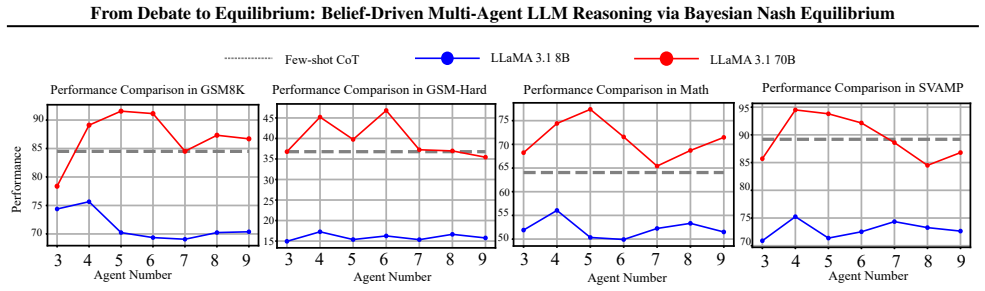
The central claim, stated on the paper's own terms, is that multi-LLM coordination can be recast as the pursuit of a Bayesian Nash equilibrium in an incomplete-information game, and that doing so yields both a convergence guarantee and better answers at lower cost than message-passing debate. Each execution LLM's belief network maps its local history to a prompt embedding — the temperature and repetition penalty of its sampler — plus a local Q-value; a belief encoder fuses all agents' belief states, and a centralized mixing network trains the local networks so that the global objective improves whenever any local policy improves. The paper proves BNE existence by Glicksberg's fixed point theorem, derives the sublinear Bayesian regret bound $O(N\sqrt{T}/(1-\gamma))$ through a performance-difference lemma with Q-estimation and policy-suboptimality error terms, and contrasts it with a linear $\Omega(NT/(1-\gamma))$ lower bound for debate settings where agents must randomize to avoid exploitation. Empirically it reports an average improvement of 10.9% over single-agent baselines and 11.2% over existing multi-LLM methods across six benchmarks, a 21.4% token reduction versus three-round debate, and an 18.1% further gain when scaling to nine execution LLMs under a hierarchy of coordinators.
Load-bearing premise
Everything rests on the unmeasured premise that the small belief networks learn the way textbook Q-learners do — their Q-value estimates and policy choices improving as $O(1/\sqrt{t})$ — even though these networks only set a temperature and a repetition penalty while a frozen LLM writes the actual answer, and that each model's guesses about its teammates' behavior stay close to the coordinator's own assessment.
Editorial extensions
If this is right
- Multi-LLM ensembles can be scaled to at least nine agents with only moderate added cost: adding two local coordinators and a central coordinator yields an 18.1% gain over the three-execution-LLM baseline.
- Token budgets fall because execution models never see one another's outputs; the paper reports 21.4% fewer tokens than a three-round debate at equal or higher accuracy.
- Cooperative belief coordination, unlike competitive debate, is claimed to carry a sublinear $O(N\sqrt{T}/(1-\gamma))$ regret bound, meaning repeated application converges toward a stable strategy profile instead of cycling.
- The framework is model-agnostic across open-weight models from 7B to 405B and GPT-4-Turbo, and heterogeneous execution teams still beat the few-shot CoT baseline, though they reach equilibrium less easily than homogeneous teams.
Reading between the lines
- Because the belief network learns only a temperature and a repetition penalty while the LLM stays frozen, the mechanism is essentially adaptive prompt-shaping; the same coordinator–belief architecture could plausibly steer any stochastic text generator toward consensus, not just LLMs.
- The paper reports that adding direct inter-agent communication to ECON raised accuracy by only 1.1% while increasing token use by 42.4%, which suggests the practical value of belief coordination is mostly cost reduction; a natural comparison is a non-learned baseline that simply averages answers sampled under a fixed temperature schedule with the same coordinator prompts.
- If the asserted $O(1/\sqrt{t})$ error decay were verified empirically, the regret framework would transfer to other hierarchical coordinator–executor designs, implying that partial observability does not block equilibrium-based coordination as long as some central belief aggregator exists.
Editorial analysis
A structured set of objections, weighed in public.
Referee Report
Summary. The paper proposes ECON, a hierarchical multi-LLM reasoning framework that replaces explicit inter-agent debate with belief-based coordination. Each execution LLM maintains a belief network that outputs a temperature and repetition penalty, and a centralized mixing network coordinates these local components. The authors claim to formalize multi-LLM coordination as a Bayesian Nash equilibrium problem, to prove BNE existence and convergence, to derive a sublinear regret bound O(N sqrt(T)/(1-gamma)) for ECON versus linear regret for multi-agent debate, and to show consistent empirical gains across six benchmarks with reduced token usage. The appendix contains the theoretical proofs, assumptions, experimental details, and tutorial-style examples.
Significance. If the theoretical and empirical claims were both established, this would be a valuable contribution: a communication-free coordination mechanism for LLM ensembles with convergence guarantees and measured efficiency gains. The paper has notable strengths: the code is public, the experiments cover several models and datasets, the scalability study is informative, and the ablation studies test some design choices. However, the central theoretical results are not supported as stated. The BNE convergence proof is circular, the regret analysis relies on an invalid learning-rate schedule and unverified regularity assumptions, and the BNE existence proof imposes conditions that do not hold for the implemented discrete-text LLM system. The headline empirical improvement is also not backed by the reported aggregate numbers. The significance of the paper therefore rests on claims that the manuscript does not justify.
major comments (5)
- [Appendix B.2, Steps 3-5] The convergence-to-BNE proof assumes that a zero gradient of the TD loss holds only when Q_i(s,a;theta*_i) = r_i + gamma max_{a'} Q_i(s',a';theta^-_i), and then uses this Bellman optimality condition to conclude that agents are best-responding. This assumption is essentially the conclusion being proved. For the neural Q-networks and belief networks actually used, a stationary point of the TD objective characterizes a projected Bellman fixed point, not global optimality, and the paper provides neither proof nor measurement that the stronger condition holds. Consequently the claimed convergence to BNE is not established, and the regret decomposition in Appendix C.2, which benchmarks against V* under the BNE, lacks a valid target.
- [Appendix C.2.3, Lemmas C.1-C.2] The proof of the O(N sqrt(T)/(1-gamma)) bound invokes Robbins-Monro conditions (sum eta_t = infinity and sum eta_t^2 < infinity) while choosing eta_t = eta_0/sqrt(t); this schedule has divergent sum eta_t^2, so the cited stochastic approximation theorem does not apply as stated. Moreover, the O(1/sqrt(t)) rates for Q-function estimation and policy suboptimality are asserted for belief networks that output only temperature and repetition penalty while the LLM produces discrete text; no argument connects neural-network TD learning or online convex optimization in the action-embedding space to the stochastic LLM generation process. The central regret bound is therefore unsupported.
- [Appendix B.1, Theorem 2.1] The BNE existence proof assumes payoff functions are continuous and quasi-concave in actions, but in the implemented system actions are prompt embeddings mapped through an LLM to discrete text, and rewards are computed on text outputs; continuity and quasi-concavity are not established and are implausible for this mapping. The proof's statement that 'strategies are linear in the space of mixed strategies' does not imply quasi-concavity of the payoff. Thus the existence theorem is not proven for the stated setting.
- [Appendix B.3 and Appendix C.3] The regret and convergence claims depend on assumptions B.4, B.6, and B.8 (approximate posterior alignment, game regularity, and concentrability), none of which are measured, derived from the ECON architecture, or otherwise justified. Similarly, the comparison with multi-agent debate in Appendix C.3 models debate as zero-sum with persistent suboptimality, but this model is not shown to describe the MAD baseline used in the experiments. The claimed linear-versus-sublinear gap is therefore not established.
- [Abstract and Section 4.2] The headline claim that ECON outperforms existing multi-LLM approaches by 11.2% on average across six benchmarks is not supported by the numbers reported in Section 4.2: the listed improvements of 25.6%, 6.3%, 10.9%, 11.2%, and 6.4% are against different baselines (zero-shot CoT, few-shot CoT, SC, ToT, rStar), not an average over existing multi-LLM approaches, and no aggregate comparison with error bars is provided. The benchmark count is also inconsistent: the paper says six benchmarks but reports five reasoning datasets plus TravelPlanner.
minor comments (5)
- [Appendix A and Section 2.2] The symbol theta_i is used both for agent types in the BNE proof and for network parameters elsewhere; this collision makes several formulas ambiguous and should be fixed.
- [Figure 3] The method label 'EcoNash' in Figure 3 differs from the name ECON used throughout the text; the axis labels are also visually corrupted and should be regenerated.
- [Figures 9-13] The accuracy comparison figures in the appendix render as hexadecimal/unicode strings rather than readable values, so the per-dataset results cannot be verified from the appendix.
- [Various] There are several small typos and inconsistencies: 'SV AMP' should be 'SVAMP', 'GPT4 turbo)' has a stray parenthesis, and Appendix B.4 refers to 'Appendix 2' instead of a proper section.
- [Appendix C.1] The proof of Lemma 2.2 states that the difference in state distributions is 'negligible (justified under Assumption B.8)', but Assumption B.8 is a concentrability condition, not an equality of state distributions; this step should be made explicit or removed.
Circularity Check
The BNE-convergence proof in Appendix B.2 assumes Bellman optimality to conclude best response, and the regret bound inherits an assumed O(1/√t) rate that is not established.
-
self definitional
[Appendix B.2, Step 3 (Proof of Convergence to BNE)]
"Assuming that the Q-network parameterization is such that the above condition holds only when: Qi(s, ai; θ∗i ) = ri + γ max a′ i Qi(s′, a′ i; θ− i ), the Q-network accurately estimates the expected cumulative rewards, aligning the agent’s policy with the optimal response to other agents’ strategies."
The proof aims to show that SGD on the TD loss drives agents to a BNE, meaning every agent is best-responding. At a stationary point of the TD loss, the zero-gradient condition for a nonlinear Q-network is a projected Bellman fixed point, not global Bellman optimality. The inserted 'only when' clause simply assumes the Bellman optimality equation, which is precisely the best-response property needed. Step 4 then restates this assumed equation as 'the Q-network satisfies the Bellman optimality condition,' and Step 5 concludes the policies form a BNE. The conclusion is therefore an input to the proof.
-
fitted input called prediction
[Appendix C.2.3, Lemma C.1, and Appendix C.2.6]
"Consider the Q-learning update rule with learning rate ηt = η0/√t: ... Lemma C.1 (Q-function Convergence Rate). Under the following conditions: (i) Learning rate schedule ηt = η0/√t ... (iii) Standard stochastic approximation conditions (Robbins-Monro) ... The Q-function estimation error satisfies: E[ϵt(s, a)] ≤ C1/√t."
The advertised O(N√T/(1−γ)) regret bound is obtained by substituting assumed rates ϵt = O(1/√t) and δt = O(1/√t) into the Q-value decomposition. The proof of Lemma C.1 does not supply this rate: it invokes Robbins-Monro conditions while using ηt = η0/√t, for which Σ ηt² diverges, so the cited stochastic approximation theorem cannot be applied as stated. The final regret bound is thus the assumed decay rate summed over T, i.e., the prediction is forced by the input rather than derived from the ECON learning dynamics.
full rationale
The empirical evaluation of ECON is not circular: it is carried out against public benchmarks and standard baselines, and no load-bearing self-citation chain was found. The central theoretical claim, however, is circular in a key step. Appendix B.2 derives convergence to BNE by assuming that the Q-network stationary point satisfies the Bellman optimality equation, which is exactly the best-response condition from which a BNE is declared. The regret analysis then inherits this: V* is defined as the BNE value, and the O(N√T/(1−γ)) bound is assembled from assumed O(1/√t) estimation and suboptimality rates, with Lemma C.1 relying on Robbins-Monro conditions violated by the paper's own ηt = η0/√t schedule. The claimed advantage over multi-agent debate is therefore not established by the supplied derivation. This corresponds to partial circularity of the central theoretical result while the empirical contribution remains independent, giving a score of 6.
Assumptions & free parameters
free parameters (4)
- Reward weights α1, α2, α3 =
0.4/0.4/0.2 (8B/70B), 0.3/0.5/0.2 (405B)
- Temperature and repetition penalty bounds Tmin/Tmax, pmin/pmax =
0.1/2.0, 0.1/0.9
- Early stopping thresholds εC, εL, Rthreshold =
0.01, 1e-4, 0.7
- Loss weights λb, λ, λm =
0.1, 0.1, 0.1
assumptions (6)
- standard math Glicksberg's fixed point theorem guarantees BNE existence for continuous, quasi-concave games.
- ad hoc to paper Assumption B.4: approximate posterior alignment, D_KL(P_LLM || P_post) ≤ ε.
- ad hoc to paper Assumption B.6: game regularity inequality on belief entropy and mutual information.
- domain assumption Assumption B.8: concentrability condition bounding cumulative Bellman error.
- ad hoc to paper Appendix B.2 Step 3: the Q-network is optimal at any stationary point of the TD loss.
- ad hoc to paper Q-function estimation error and policy suboptimality decay as O(1/√t).
invented entities (1)
-
Belief state bi (latent coordination variable)
Cite this review
Pith. "Pith review of From Debate to Equilibrium: Belief-Driven Multi-Agent LLM Reasoning via Bayesian Nash Equilibrium." pith.science (2026). https://pith.science/paper/K7RYTIVO
@misc{pith2026250608292,
  author       = {Pith},
  title        = {Pith review of: From Debate to Equilibrium: Belief-Driven Multi-Agent LLM Reasoning via Bayesian Nash Equilibrium},
  year         = {2026},
  howpublished = {\url{https://pith.science/paper/K7RYTIVO}},
  note         = {Machine review of arXiv:2506.08292}
}
read the original abstract
Multi-agent frameworks can substantially boost the reasoning power of large language models (LLMs), but they typically incur heavy computational costs and lack convergence guarantees. To overcome these challenges, we recast multi-LLM coordination as an incomplete-information game and seek a Bayesian Nash equilibrium (BNE), in which each agent optimally responds to its probabilistic beliefs about the strategies of others. We introduce Efficient Coordination via Nash Equilibrium (ECON), a hierarchical reinforcement-learning paradigm that marries distributed reasoning with centralized final output. Under ECON, each LLM independently selects responses that maximize its expected reward, conditioned on its beliefs about co-agents, without requiring costly inter-agent exchanges. We mathematically prove that ECON attains a markedly tighter regret bound than non-equilibrium multi-agent schemes. Empirically, ECON outperforms existing multi-LLM approaches by 11.2% on average across six benchmarks spanning complex reasoning and planning tasks. Further experiments demonstrate ECON's ability to flexibly incorporate additional models, confirming its scalability and paving the way toward larger, more powerful multi-LLM ensembles. The code is publicly available at: https://github.com/tmlr-group/ECON.
Figures


Figures from the paper (11 more)


Reference graph
Works this paper leans on
-
[1]
Strategy Space Compactness and Convexity: • The strategy space Πi is non-empty, convex, and compact in the topology of pointwise convergence
-
[2]
Continuity of Payoff Functions: • The payoff function Ui(θi, πi, π−i) is continuous in (πi, π−i) for each fixed θi
-
[3]
Quasi-Concavity of Payoff Functions: • The payoff function Ui(θi, πi, π−i) is quasi-concave in πi for each fixed θi and π−i. Verification:
-
[4]
Strategy Space Compactness and Convexity: The strategy space Πi consists of all measurable functions mapping types θi to actions ai in Ai. Since Θi and Ai are compact metric spaces, and strategies are measurable functions from one compact space to another, the space of such functions Πi can be endowed with the topology of pointwise convergence, making it ...
-
[5]
Continuity of Payoff Functions: For fixed θi, the payoff function Ui(θi, πi, π−i) depends continuously on πi and π−i due to the continuity of Ui in actions and types. Specifically, since Ui is continuous in a = (ai, a−i) and the strategies πi, π−i map continuously from types to actions, the composition Ui(θi, πi(θi), π−i(θ−i)) is continuous in (πi, π−i)
-
[6]
Quasi-Concavity of Payoff Functions: For each θi and π−i, the function πi 7→ Ui(θi, πi, π−i) is quasi-concave because Ui is quasi-concave in ai and the strategies are linear in the space of mixed strategies. Therefore, any convex combination of strategies does not decrease the utility, satisfying quasi-concavity. Step 3: Establish Upper Hemicontinuity and...
-
[7]
Non-Empty, Convex Values: For each π−i, since Πi is compact and convex, and Ui is continuous and quasi-concave in πi, the Weierstrass Theorem ensures that the maximum exists; hence, BRi(π−i) is non-empty. Convexity follows from the quasi-concavity of Ui in πi, implying that any convex combination of best responses is also a best response. 16 From Debate t...
-
[8]
Upper Hemicontinuity: Upper hemicontinuity of BRi means that for any net πα −i → π−i, and any πi ∈ BRi(π−i), there exists a net πα i ∈ BRi(πα −i) such that πα i → πi. This property holds because the payoff function Ui is continuous in (πi, π−i), and the strategy spaces are compact. Step 4: Application of Glicksberg’s Fixed Point Theorem Having verified al...
Show all 53 references
-
[9]
The Q-networks Qi(s, ai; θi) are parameterized by prompt embeddings θi, and the mapping from θi to Qi is continu- ously differentiable
-
[10]
The exploration strategy ensures sufficient coverage of the state-action space (e.g., ϵ-greedy with decaying ϵ)
-
[11]
The loss function Li(θi) is convex or has Lipschitz continuous gradients with respect to θi
-
[12]
The gradient ∇θi Li(θi) is Lipschitz continuous
-
[13]
∞X k=0 γkri(sk, ak) | s0 = s # , V π i (s) = Eπ
The learning rate ηt is chosen such that it satisfies the Robbins-Monro conditions: P∞ t=1 ηt = ∞ and P∞ t=1 η2 t < ∞. Step 1: Defining the TD Loss Function The TD loss function for agent i is: Li(θi) = E(s,ai,ri,s′)∼Di " ri + γ max a′ i Qi(s′, a′ i; θ− i ) − Qi(s, ai; θi) 2# ...
2009
-
[14]
Strategic Cycling: Agents continuously adapt to opponents, preventing convergence to optimal deterministic policies
-
[15]
Exploration-Exploitation Conflict: Need for defensive randomization conflicts with exploitation of learned knowledge
-
[16]
Information Inefficiency: Lack of coordination prevents efficient use of collective information In contrast, ECON’s cooperative framework with Bayesian policy optimization enables agents to: • Share information through the communication phase • Coordinate strategies toward Bay...
2023
-
[17]
This is a textual or embedded summary of the agent’s partial view of the environment, updated via the belief network
Local Belief State bt i. This is a textual or embedded summary of the agent’s partial view of the environment, updated via the belief network
-
[18]
Figure 6: Coordinator Prompt(for Strategy)
Coordinator Strategy es. The high-level guidance from the Coordinator LLM. If the total token count (prompt + expected output) could exceed the Together API’s per-request cap (e.g., 2048 tokens), we truncate repeated instructions or compress partial states. Similarly, we impos...
-
[19]
If Tom saves $45 per week, how much does Janet save in 5 weeks? S2: Find Janet’s weekly savings relative to Tom’s
Total = subtotal + tip Strategy + F ormat: 35tokens GSM8K Problem 2: Q2: Janet saves twice as much money as Tom. If Tom saves $45 per week, how much does Janet save in 5 weeks? S2: Find Janet’s weekly savings relative to Tom’s. Multiply by number of weeks. F2:
-
[20]
Janet weekly = ? × Tom
-
[21]
If they increase production by 15% next month, how many cars will they produce in a 30-day month? S3: Calculate production increase
Total = weekly × weeks Strategy + F ormat: 28tokens 37 From Debate to Equilibrium: Belief-Driven Multi-Agent LLM Reasoning via Bayesian Nash Equilibrium GSM8K Problem 3: Q3: A factory produces 150 cars per day. If they increase production by 15% next month, how many cars will ...
-
[22]
Increase = original × 15%
-
[23]
New daily = original + increase
-
[24]
Sarah then gives 1 4 of her marbles to Tom
Monthly = daily × days Strategy + F ormat: 36tokens GSM8K Problem 4: Q4: Alex has 240 marbles and gives 3 8 of them to Sarah. Sarah then gives 1 4 of her marbles to Tom. How many marbles does Sarah have left? S4: Calculate Sarah’s initial share. Find amount she gives to Tom. S...
-
[25]
Sarah gets = total × 3 8
-
[26]
Sarah gives = her marbles × 1 4
-
[27]
What’s the total distance traveled? S5: Calculate distance for each speed separately using d = r × t
Remaining = initial - given Strategy + F ormat: 39tokens GSM8K Problem 5: Q5: A train travels at 60 mph for 2.5 hours, then increases speed to 75 mph for 1.5 hours. What’s the total distance traveled? S5: Calculate distance for each speed separately using d = r × t. Sum distances. F5:
-
[28]
First distance = speed 1 × time1
-
[29]
Second distance = speed 2 × time2
-
[30]
MATH MATH Problem 1: Q1: In a bag of marbles, 3 7 are blue and 2 5 are red
Total = d1 + d2 Strategy + F ormat: 36tokens F.2.2. MATH MATH Problem 1: Q1: In a bag of marbles, 3 7 are blue and 2 5 are red. The remaining 11 marbles are green. How many marbles are in the bag? S1: Convert fractions to common denominator. Find the fraction for remaining col...
-
[31]
Convert to common denominator
-
[32]
Add converted fractions
-
[33]
S2: Use coordinate geometry method for area
Use remaining count to find total Strategy + F ormat: 32tokens MATH Problem 2: Q2: Find the area of a triangle with vertices at (0,0), (4,0), and (2,5). S2: Use coordinate geometry method for area. Set up calculation matrix. Take final result. F2:
-
[34]
Set up coordinate matrix
-
[35]
Calculate determinant
-
[36]
S3: Apply logarithm properties
Apply area formula Strategy + F ormat: 28tokens 38 From Debate to Equilibrium: Belief-Driven Multi-Agent LLM Reasoning via Bayesian Nash Equilibrium MATH Problem 3: Q3: If log2(x) = 3and log2(y) = 4, find log2(xy). S3: Apply logarithm properties. Combine given values. Express ...
-
[37]
Write multiplication property
-
[38]
Substitute given values
-
[39]
Find the area of the sector formed by a 40◦ angle at the center
Simplify result Strategy + F ormat: 26tokens MATH Problem 4: Q4: A circle has radius 6. Find the area of the sector formed by a 40◦ angle at the center. S4: Convert angle measurement. Apply sector area formula. Simplify result. F4:
-
[40]
Write sector formula
-
[41]
S5: Identify quadratic components
Calculate final area Strategy + F ormat: 27tokens MATH Problem 5: Q5: Solve the equation: 2x2 + 5x − 12 = 0. S5: Identify quadratic components. Apply standard formula. Solve for variables. F5:
-
[42]
Identify coefficients
-
[43]
Setup quadratic formula
-
[44]
SVAMP SV AMP Problem 1: Q1: There are 56 books on the shelf
Calculate solutions Strategy + F ormat: 28tokens F.2.3. SVAMP SV AMP Problem 1: Q1: There are 56 books on the shelf. Tom puts 14 more books and Jane removes 22 books. How many books are on the shelf now? S1: Track sequential changes. Apply additions and subtractions in order. F1:
-
[45]
Each row has 4 chocolates
Subtract removed books Strategy + F ormat: 25tokens SV AMP Problem 2: Q2: A box has 3 rows of chocolates. Each row has 4 chocolates. If 5 chocolates were eaten, how many are left? S2: Calculate initial total. Subtract consumed amount. F2:
-
[46]
Find total chocolates
-
[47]
John has 12 stickers
Subtract eaten ones Strategy + F ormat: 23tokens 39 From Debate to Equilibrium: Belief-Driven Multi-Agent LLM Reasoning via Bayesian Nash Equilibrium SV AMP Problem 3: Q3: Mary has 5 times as many stickers as John. John has 12 stickers. How many stickers do they have together?...
-
[48]
Find Mary’s stickers
-
[49]
( 2 7 ) are roses and ( 3 7 ) are tulips
Add both totals Strategy + F ormat: 24tokens SV AMP Problem 4: Q4: A garden has 35 flowers. ( 2 7 ) are roses and ( 3 7 ) are tulips. How many flowers are neither roses nor tulips? S4: Sum known fractions. Find remaining fraction. Calculate final count. F4:
-
[50]
Find remaining fraction
-
[51]
If there are 23 children, how many boxes of 10 pencils should the teacher buy? S5: Calculate total need
Calculate flower count Strategy + F ormat: 27tokens SV AMP Problem 5: Q5: Each child needs 3 pencils. If there are 23 children, how many boxes of 10 pencils should the teacher buy? S5: Calculate total need. Convert to required units. Round appropriately. F5:
-
[52]
Calculate total pencils
-
[53]
Round to whole boxes Strategy + F ormat: 28tokens Note on Token Counts: • All problems follow consistent format: strategy + step-by-step format • Strategy statements aim to be concise yet clear • Format points provide framework without giving solutions • Token ranges: – Shorte...
Reviewed August 7, 2026 · model on record in the stance chip above.
Discussion (0). Sign in to comment.