REVIEW 4 major objections 4 minor 43 references
How to Provably Improve Return Conditioned Supervised Learning?
T0 review · 4 major / 4 minor · reviewed 2026-08-07 · deepseek-v4-flash
Pith's one-line read Provable stitching for return-conditioned reinforcement learning, without dynamic programming.
desk verdict Genuine deterministic-environment results for RCSL stitching, but the central theorem's stochastic claim is unsupported by its own proof; a fixable overreach that still deserves peer review. read the letter →
The pith
A machine-rendered reading of the paper's core claim, the machinery that carries it, and where it could break.
The reading
What carries the argument
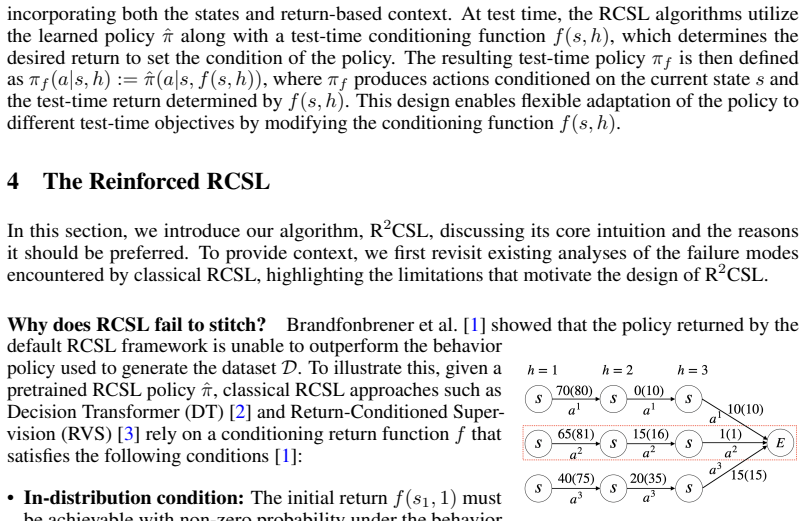
The load-bearing object is the in-distribution optimal return-to-go, $f^\star(s,h) := \arg\max_{f \in \mathcal{F}_\beta(s,h)} f(s,h)$, i.e., the largest return-to-go that appears in any trajectory of the behavior policy passing through state $s$ at stage $h$. The in-distribution optimal stitched policy is $\pi^\star_\beta(a|s,h) := P_\beta(a|s,h,f^\star(s,h))$: the behavior policy's action distribution conditioned on that maximal achievable return. It carries the argument because conditioning on $f^\star$ at each step lets the policy select the best future from whichever trajectory offers it, without ever querying an out-of-distribution return. A second mechanism is the relabeling rule $\tilde{g}^k_h = \max\{ r_h + f^\star_{k-1}(s_{h+1},h+1),\, r_h + \tilde{g}^k_{h+1} \}$, which propagates best future returns backward; after $H-1$ passes it yields $Q^{\star,\beta}_h(s_h,a_h)$ in deterministic environments, showing the gap to dynamic programming closes.
What would settle it
Construct a two-stage MDP with a single start state $s_1$, reward $r(s_1,a)=0$, and two actions: action $L$ leads with probability 0.5 to a state with max return-to-go 10 and with probability 0.5 to a state with max return-to-go 0; action $R$ leads deterministically to a state with max return-to-go 9. Then $f^\star(s_1,1)=10$ via action $L$, so the policy $\pi^\star_\beta$ conditions on 10 and its expected return is $0.5\cdot 10 + 0.5\cdot 0 = 5$, which is below $J(\pi_f)=9$ for the consistent $f$ that picks action $R$. This directly contradicts Theorem 4.1's inequality in a stochastic environment.
Extended reading notes
Core claim
The paper's core discovery is that the ceiling RCSL inherits from the dataset comes from the consistency condition on the conditioning function $f$, not from supervised learning itself. By defining $f^\star(s,h)$ as the maximum return-to-go over all conditioning functions that are feasible under the behavior policy—that is, the best future return that occurs in any dataset trajectory through $(s,h)$—and conditioning the learned policy on $f^\star$, the induced policy $\pi^\star_\beta$ is proved to satisfy $J(\pi^\star_\beta) \ge J(\pi_f)$ for every consistent $f$ (Theorem 4.1). This is the first proof that an RCSL-style method can stitch: combine pieces of different trajectories to exceed the best trajectory in the data. Finite-sample versions show R2CSL converges to $\pi^\star_\beta$ at rate $N^{-1/4}$ with the same coverage assumptions as ordinary RCSL (Theorem 5.3), and with quantile regression the in-distribution optimal RTG is recovered exactly once the dataset covers it (Theorem 6.2).
Load-bearing premise
For the main domination theorem, the proof assumes deterministic transitions, so that $f^\star(s,h)$ is actually achievable by the policy that conditions on it; if the environment branches stochastically, the policy can fail to realize the max return-to-go it was told to aim for.
Editorial extensions
If this is right
- R2CSL policies can exceed the best trajectory in the dataset by stitching together high-return segments from different trajectories, breaking the ceiling that ordinary RCSL inherits.
- The improvement comes at the same sample-complexity order as classical RCSL: the $N^{-1/4}$ rate and the coverage constants $c^\star_\beta$ and $\tilde{c}$ play the same roles as the corresponding terms in the prior RCSL analysis.
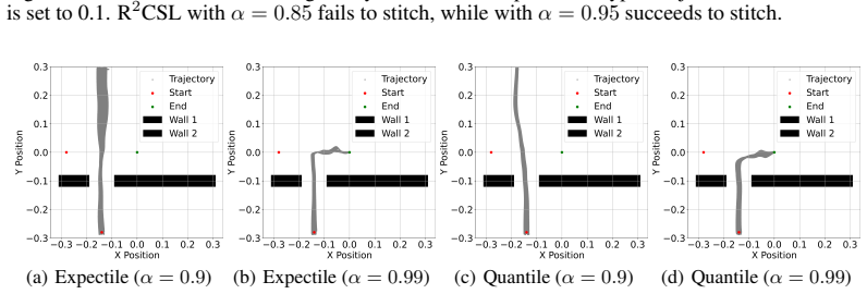
- Quantile regression, not expectile regression, is the correct estimator for the optimal RTG: with enough data it recovers $f^\star$ exactly, while expectile regression can learn out-of-distribution returns and fail.
- The multi-step relabeling variant achieves the in-distribution optimal policy after $H-1$ passes, so RCSL-style methods can match dynamic-programming-based methods' guarantee in deterministic settings.
- The framework is flexible enough to be layered onto RvS, DT, and QT-style architectures, improving each in the reported benchmarks.
Reading between the lines
- The domination theorem is proven under deterministic transitions; in stochastic environments the conditioning function $f^\star(s,h)$ can exceed the return any policy can guarantee, so the practical gains in stochastic benchmarks likely rest on the policy's ability to hedge rather than on Theorem 4.1 itself.
- The relabeling rule (8.1) suggests a natural stochastic extension: replace the max with an expectile or quantile of the next-state value and test whether the $H-1$-pass optimality persists with a risk-sensitive objective.
- Since the only role of $f^\star$ is to pick the strongest feasible conditioning signal, the same construction could be applied to goal-conditioned supervised learning, where the “return” is a goal-achievement score rather than cumulative reward.
Editorial analysis
A structured set of objections, weighed in public.
Referee Report
Summary. The paper proposes Reinforced RCSL (R2CSL), an offline RL method that conditions a return-conditioned supervised learning policy on an "in-distribution optimal RTG" f*(s,h) defined as the maximum return-to-go achievable under the behavior policy's feasible trajectory set. The central theoretical claim (Theorem 4.1) is that the resulting policy pi*_beta dominates every consistent RCSL policy pi_f, providing a provable stitching guarantee without dynamic programming. The paper gives finite-sample bounds for a tabular deterministic setting (Theorem 5.3) and a general stochastic setting with function approximation (Theorem 5.5), analyzes expectile versus quantile regression for estimating f* (Section 6), and proposes a multi-step relabeling scheme claimed to recover the optimal in-distribution policy (Theorem 8.1). Experiments on PointMaze, D4RL Gym, and AntMaze report improvements over RvS and DT baselines.
Significance. If the main claim is correct in the stated generality, this would be the first provable stitching guarantee for RCSL that avoids dynamic programming, a significant conceptual contribution to offline RL theory. The paper also provides a useful comparison of expectile and quantile estimators for the conditioning function and shows that quantile regression can recover the in-distribution maximum RTG in a deterministic tabular setting. The empirical study is reasonably broad, and the theoretical results, while building on existing RCSL analysis, address a real gap. However, the central domination claim is currently proven only under deterministic transitions, and the stochastic analysis does not establish that R2CSL dominates consistent RCSL policies in stochastic environments.
major comments (4)
- [Theorem 4.1 and Appendix A.1] Theorem 4.1 is stated for general MDPs, but the proof in Appendix A.1 is explicitly deterministic. The proof reasons about 'the state transitioned from s by taking a*_1' as a single state, which is only valid when P(s'|s,a) is deterministic. In a stochastic MDP, after selecting the action realizing f*(s,h), the next state s' is random, and f*(s',h+1) can be strictly smaller than f*(s,h)-r. Consequently the chain J(pi*_beta) >= E[f(s,1)] >= J(pi_f) breaks at the first inequality. The theorem as stated is therefore unsupported; the paper should either restrict Theorem 4.1 to deterministic environments or provide a genuinely stochastic proof with appropriate assumptions.
- [Section 5.2 and Theorem 5.5] The stochastic analysis does not repair the gap in Theorem 4.1. Theorem 5.5 only bounds J(pi*_beta) - J(hat_pi*_D), the error relative to the in-distribution optimal stitched policy pi*_beta. It does not show that pi*_beta dominates all consistent RCSL policies in stochastic environments; indeed the paper itself concedes in Section 9 that such objective policies 'can be arbitrarily suboptimal' and cites prior work to this effect. Thus the central contribution, 'provably improve RCSL,' is established only for deterministic transitions. The authors should clearly state this limitation in the abstract and introduction, or extend the analysis.
- [Appendix A.6, Theorem 8.1] The proof of Theorem 8.1 is informal and narrative rather than a rigorous induction. It asserts that after H-1 relabeling passes one has ~g^{H-1}_h = Q*_beta_h(s_h,a_h), but the argument is a sequence of case discussions ('Q1', 'Q2', 'case (i)', 'case (ii)') without a formal inductive hypothesis or a precise definition of what dataset distribution the relabeled trajectories induce. Since Theorem 8.1 supports the claim of closing the gap with dynamic programming, it needs a complete proof or an explicit label as a proof sketch, with the formal details supplied in an appendix.
- [Section 6, Theorem 6.2 proof] The proof of Theorem 6.2 in Appendix A.5 shows that the number of samples at f*(s,h) is large and concludes that the alpha-quantile equals f*(s,h). This relies on the deterministic, no-tie assumption in Assumption 6.1, which is stated, but the proof does not explicitly handle the case where multiple actions or trajectories attain the conditioning value, nor does it connect the empirical quantile from the L1 loss to the population quantile under the assumed coverage. A precise statement of why the finite-sample quantile estimate coincides with f* with high probability would strengthen the result; currently the proof is incomplete at the step 'then setting alpha > 1 - c~/2, the alpha-quantile is exactly f*(s,h)'.
minor comments (4)
- [Section 6, before Theorem 6.2] In the sentence 'We set α > 1−˜c/2 in the Lα2 loss with quantile regression', the quantile loss is L1, not Lα2; the notation should be corrected.
- [Sections 5.1 and 5.2] Theorems are referenced inconsistently: 'Assume Theorems 5.1 and 5.2 hold' should read 'Assumptions 5.1 and 5.2'; likewise 'satisfy Theorem 5.4' should be 'Assumption 5.4'. This makes the logical dependencies harder to follow.
- [Appendix A.1] The proof of Theorem 4.1 says 'By Corollary 2 of [1], we have J(pi^{RCSL}_f) = E[f(s,1)]' and later 'it is trivial that the trajectory induced by pi* is better', but the deterministic argument is not written in formal notation; a concrete induction on h would significantly improve clarity.
- [Section 7.1, Figure 4 caption] The text states that with 1% Type I trajectories α=0.90 fails, but the caption of Figure 4 mentions α=0.85 for the failure case; please align the caption with the main text.
Circularity Check
Theorem 4.1's claimed provable improvement over RCSL is partially self-definitional: f* is defined as the pointwise maximum over the same feasible conditioning set, so the initial-return dominance over consistent f is built into Eq. (4.1).
-
self definitional
[Section 4.1, Eq. (4.1), Theorem 4.1 and Appendix A.1]
"f⋆(s, h) := argmax_{f∈Fβ(s,h)} f(s, h) ... π⋆β(a|s, h) := Pβ(a|s, h, f⋆(s, h)) ... Theorem 4.1. For any f∈F Cst β, we have J(π⋆β)≥J(πf). Proof: 'By Corollary 2 of [1], we have J(π RCSL f)=E s∼ρ[f(s,1)] ... it is trivial that the trajectory induced by π⋆ is better than the trajectory in ˜T1(s).'"
The dominance is built into the definition: f* is the pointwise maximum over the same feasible set F_β whose consistent members f∈F_Cst^β are the comparison class, so f*(s,1)≥f(s,1) for every consistent f by construction. After invoking [1]'s equality J(π_f^RCSL)=E[f(s,1)], the only remaining content is whether π*_β actually achieves the return f*(s,1); the proof asserts this via 'the equivalence of the conditioning function and the set of trajectories' in a deterministic argument (Appendix A.1). Thus the 'provable improvement over RCSL' is, at the initial-state level, the tautology that the maximum feasible return is at least any feasible return, plus an achievability assumption that is stated rather than proven in stochastic environments.
full rationale
The only reduction I can exhibit with the paper's own equations is in the headline domination claim. Eq. (4.1) defines f*(s,h) as the maximum over the feasible conditioning set F_β(s,h), and the comparison class in Theorem 4.1 is the consistent subset F_Cst^β ⊂ F_β. Hence f*(s,1) ≥ f(s,1) for every consistent f by construction. The proof then relies on [1]'s equality J(π_f^RCSL)=E[f(s,1)] and asserts that π*_β realizes f* ('the trajectory induced by π⋆ is better than the trajectory in ˜T1(s)'; the deterministic reasoning in Appendix A.1). So the 'provable improvement over standard RCSL' rests on a definitional maximum plus an achievability assertion rather than on an independently derived bound; this is partial circularity. The sample-complexity theorems (5.3, 5.5, 6.2), the quantile-regression analysis, and the D4RL experiments are not circular: they compare against external benchmarks and use standard MLE-concentrability arguments, and [1] is an external citation, not a self-citation. I also note the paper itself concedes in Section 9 that RCSL-style objective policies 'can be arbitrarily suboptimal' in stochastic environments; the stochastic proof of Theorem 5.5 only estimates π*_β and does not repair the deterministic achievability gap in Theorem 4.1. This is a correctness limitation rather than an additional circular step, so it does not change the score beyond the partial definitional dominance already counted.
Assumptions & free parameters
free parameters (2)
- alpha (expectile/quantile level) =
0.9, 0.99, 0.999 in experiments; theory requires alpha > 1 - c_tilde/2
- Number of relabeling passes k =
H-1 in Theorem 8.1; not tuned in experiments
assumptions (6)
- standard math Finite policy class with bounded log-likelihood ratio and bounded approximation error (Assumption 5.1)
- domain assumption Return coverage: P_beta(g_h = f*(s,h) | s_h=s) >= c_tilde for all (s,h) in dom(f*) (Assumption 5.2)
- domain assumption Distribution mismatch: d^{*,beta}_h(s)/d^beta_h(s) <= c*_beta (Assumption 5.2)
- domain assumption Lipschitz continuity of the policy in the conditioning RTG (Assumption 5.4)
- ad hoc to paper Deterministic transitions for the stitching argument in Theorem 4.1
- domain assumption Deterministic environment and no ties in RTG (Assumption 6.1)
Cite this review
Pith. "Pith review of How to Provably Improve Return Conditioned Supervised Learning?." pith.science (2026). https://pith.science/paper/SN4HBWKV
@misc{pith2026250608463,
  author       = {Pith},
  title        = {Pith review of: How to Provably Improve Return Conditioned Supervised Learning?},
  year         = {2026},
  howpublished = {\url{https://pith.science/paper/SN4HBWKV}},
  note         = {Machine review of arXiv:2506.08463}
}
read the original abstract
In sequential decision-making problems, Return-Conditioned Supervised Learning (RCSL) has gained increasing recognition for its simplicity and stability in modern decision-making tasks. Unlike traditional offline reinforcement learning (RL) algorithms, RCSL frames policy learning as a supervised learning problem by taking both the state and return as input. This approach eliminates the instability often associated with temporal difference (TD) learning in offline RL. However, RCSL has been criticized for lacking the stitching property, meaning its performance is inherently limited by the quality of the policy used to generate the offline dataset. To address this limitation, we propose a principled and simple framework called Reinforced RCSL. The key innovation of our framework is the introduction of a concept we call the in-distribution optimal return-to-go. This mechanism leverages our policy to identify the best achievable in-dataset future return based on the current state, avoiding the need for complex return augmentation techniques. Our theoretical analysis demonstrates that Reinforced RCSL can consistently outperform the standard RCSL approach. Empirical results further validate our claims, showing significant performance improvements across a range of benchmarks.
Figures


Figures from the paper (1 more)
Reference graph
Works this paper leans on
-
[1]
David Brandfonbrener, Alberto Bietti, Jacob Buckman, Romain Laroche, and Joan Bruna. When does return-conditioned supervised learning work for offline reinforcement learning? Advances in Neural Information Processing Systems, 35:1542–1553, 2022. 2, 3, 4, 6, 13, 17, 23
work page 2022
-
[2]
Lili Chen, Kevin Lu, Aravind Rajeswaran, Kimin Lee, Aditya Grover, Misha Laskin, Pieter Abbeel, Aravind Srinivas, and Igor Mordatch. Decision transformer: Reinforcement learning 1For two distributionsPandQ,P≪QmeansPis absolutely continuous w.r.t. Q. 13 via sequence modeling.Advances in neural information processing systems, 34:15084–15097,
-
[3]
Scott Emmons, Benjamin Eysenbach, Ilya Kostrikov, and Sergey Levine. Rvs: What is essential for offline rl via supervised learning? InInternational Conference on Learning Representations,
-
[4]
Benjamin Eysenbach, Soumith Udatha, Russ R Salakhutdinov, and Sergey Levine. Imitating past successes can be very suboptimal.Advances in Neural Information Processing Systems, 35:6047–6059, 2022. 13
work page 2022
-
[5]
D4rl: Datasets for deep data-driven reinforcement learning.arXiv preprint arXiv:2004.07219, 2020
Justin Fu, Aviral Kumar, Ofir Nachum, George Tucker, and Sergey Levine. D4rl: Datasets for deep data-driven reinforcement learning.arXiv preprint arXiv:2004.07219, 2020. 8, 23, 24
arXiv 2004
-
[6]
A minimalist approach to offline reinforcement learning
Scott Fujimoto and Shixiang Shane Gu. A minimalist approach to offline reinforcement learning. Advances in neural information processing systems, 34:20132–20145, 2021. 1
work page 2021
-
[7]
Generalized decision transformer for of- fline hindsight information matching
Hiroki Furuta, Yutaka Matsuo, and Shixiang Shane Gu. Generalized decision transformer for of- fline hindsight information matching. InInternational Conference on Learning Representations,
-
[8]
Act: empowering decision transformer with dynamic programming via advantage conditioning
Chen-Xiao Gao, Chenyang Wu, Mingjun Cao, Rui Kong, Zongzhang Zhang, and Yang Yu. Act: empowering decision transformer with dynamic programming via advantage conditioning. In Proceedings of the AAAI Conference on Artificial Intelligence, volume 38, pages 12127–12135,
Show all 43 references
-
[9]
Deepseek-r1: Incentivizing reasoning capability in llms via reinforcement learning.arXiv preprint arXiv:2501.12948, 2025
Daya Guo, Dejian Yang, Haowei Zhang, Junxiao Song, Ruoyu Zhang, Runxin Xu, Qihao Zhu, Shirong Ma, Peiyi Wang, Xiao Bi, et al. Deepseek-r1: Incentivizing reasoning capability in llms via reinforcement learning.arXiv preprint arXiv:2501.12948, 2025. 1
2025 arXiv
-
[10]
Q-value regularized transformer for offline reinforcement learning
Shengchao Hu, Ziqing Fan, Chaoqin Huang, Li Shen, Ya Zhang, Yanfeng Wang, and Dacheng Tao. Q-value regularized transformer for offline reinforcement learning. InInternational Conference on Machine Learning, pages 19165–19181. PMLR, 2024. 2, 10, 24
2024
-
[11]
Offline reinforcement learning as one big sequence modeling problem.Advances in neural information processing systems, 34:1273– 1286, 2021
Michael Janner, Qiyang Li, and Sergey Levine. Offline reinforcement learning as one big sequence modeling problem.Advances in neural information processing systems, 34:1273– 1286, 2021. 2
2021
-
[12]
Is pessimism provably efficient for offline rl? In International Conference on Machine Learning, pages 5084–5096
Ying Jin, Zhuoran Yang, and Zhaoran Wang. Is pessimism provably efficient for offline rl? In International Conference on Machine Learning, pages 5084–5096. PMLR, 2021. 1
2021
-
[13]
Reinforcement learning in robotics: A survey
Jens Kober, J Andrew Bagnell, and Jan Peters. Reinforcement learning in robotics: A survey. The International Journal of Robotics Research, 32(11):1238–1274, 2013. 1
2013
-
[14]
Quantile regression.Journal of economic perspectives, 15(4):143–156, 2001
Roger Koenker and Kevin F Hallock. Quantile regression.Journal of economic perspectives, 15(4):143–156, 2001. 2, 7
2001
-
[15]
Offline reinforcement learning with implicit q-learning
Ilya Kostrikov, Ashvin Nair, and Sergey Levine. Offline reinforcement learning with implicit q-learning. InInternational Conference on Learning Representations, 2022. 1
2022
-
[16]
Reward-conditioned policies.arXiv preprint arXiv:1912.13465, 2019
Aviral Kumar, Xue Bin Peng, and Sergey Levine. Reward-conditioned policies.arXiv preprint arXiv:1912.13465, 2019. 1
1912 arXiv
-
[17]
Conservative q-learning for offline reinforcement learning.Advances in Neural Information Processing Systems, 33: 1179–1191, 2020
Aviral Kumar, Aurick Zhou, George Tucker, and Sergey Levine. Conservative q-learning for offline reinforcement learning.Advances in Neural Information Processing Systems, 33: 1179–1191, 2020. 1, 2, 13
2020
-
[18]
Offline reinforcement learning: Tutorial, review, and perspectives on open problems.arXiv preprint arXiv:2005.01643, 2020
Sergey Levine, Aviral Kumar, George Tucker, and Justin Fu. Offline reinforcement learning: Tutorial, review, and perspectives on open problems.arXiv preprint arXiv:2005.01643, 2020. 1
2005 arXiv
-
[19]
Deep rein- forcement learning for dynamic treatment regimes on medical registry data
Ying Liu, Brent Logan, Ning Liu, Zhiyuan Xu, Jian Tang, and Yangzhi Wang. Deep rein- forcement learning for dynamic treatment regimes on medical registry data. In2017 IEEE international conference on healthcare informatics (ICHI), pages 380–385. IEEE, 2017. 1 14
2017
-
[20]
Deep spatial q- learning for infectious disease control.Journal of Agricultural, Biological and Environmental Statistics, 28(4):749–773, 2023
Zhishuai Liu, Jesse Clifton, Eric B Laber, John Drake, and Ethan X Fang. Deep spatial q- learning for infectious disease control.Journal of Agricultural, Biological and Environmental Statistics, 28(4):749–773, 2023. 1
2023
-
[21]
Human-level control through deep reinforcement learning.nature, 518(7540):529–533, 2015
V olodymyr Mnih, Koray Kavukcuoglu, David Silver, Andrei A Rusu, Joel Veness, Marc G Bellemare, Alex Graves, Martin Riedmiller, Andreas K Fidjeland, Georg Ostrovski, et al. Human-level control through deep reinforcement learning.nature, 518(7540):529–533, 2015. 1
2015
-
[22]
Asymmetric least squares estimation and testing
Whitney K Newey and James L Powell. Asymmetric least squares estimation and testing. Econometrica: Journal of the Econometric Society, pages 819–847, 1987. 2, 7
1987
-
[23]
You can’t count on luck: Why decision transformers and rvs fail in stochastic environments.Advances in neural information processing systems, 35:38966–38979, 2022
Keiran Paster, Sheila McIlraith, and Jimmy Ba. You can’t count on luck: Why decision transformers and rvs fail in stochastic environments.Advances in neural information processing systems, 35:38966–38979, 2022. 3
2022
-
[24]
Reinforcement learning upside down: Don’t predict rewards–just map them to actions.arXiv preprint arXiv:1912.02875, 2019
Juergen Schmidhuber. Reinforcement learning upside down: Don’t predict rewards–just map them to actions.arXiv preprint arXiv:1912.02875, 2019. 2
1912 arXiv
-
[25]
Reinforcement learning in robotic applications: a comprehensive survey.Artificial Intelligence Review, 55(2):945–990, 2022
Bharat Singh, Rajesh Kumar, and Vinay Pratap Singh. Reinforcement learning in robotic applications: a comprehensive survey.Artificial Intelligence Review, 55(2):945–990, 2022. 1
2022
-
[26]
Training agents using upside-down reinforcement learning.arXiv preprint arXiv:1912.02877, 2019
Rupesh Kumar Srivastava, Pranav Shyam, Filipe Mutz, Wojciech Ja ´skowski, and Jürgen Schmidhuber. Training agents using upside-down reinforcement learning.arXiv preprint arXiv:1912.02877, 2019. 2
1912 arXiv
-
[27]
MIT press,
Richard S Sutton and Andrew G Barto.Reinforcement learning: An introduction. MIT press,
-
[28]
Temporal difference learning and td-gammon.Communications of the ACM, 38(3):58–68, 1995
Gerald Tesauro et al. Temporal difference learning and td-gammon.Communications of the ACM, 38(3):58–68, 1995. 2
1995
-
[29]
Grandmaster level in starcraft ii using multi-agent reinforcement learning.nature, 575(7782):350–354, 2019
Oriol Vinyals, Igor Babuschkin, Wojciech M Czarnecki, Michaël Mathieu, Andrew Dudzik, Jun- young Chung, David H Choi, Richard Powell, Timo Ewalds, Petko Georgiev, et al. Grandmaster level in starcraft ii using multi-agent reinforcement learning.nature, 575(7782):350–354, 2019. 1
2019
-
[30]
Return augmented decision transformer for off-dynamics reinforcement learning.arXiv preprint arXiv:2410.23450, 2024
Ruhan Wang, Yu Yang, Zhishuai Liu, Dongruo Zhou, and Pan Xu. Return augmented decision transformer for off-dynamics reinforcement learning.arXiv preprint arXiv:2410.23450, 2024. 1
2024
-
[31]
Q-learning.Machine learning, 8:279–292, 1992
Christopher JCH Watkins and Peter Dayan. Q-learning.Machine learning, 8:279–292, 1992. 2
1992
-
[32]
Elastic decision transformer.Advances in Neural Information Processing Systems, 36, 2024
Yueh-Hua Wu, Xiaolong Wang, and Masashi Hamaya. Elastic decision transformer.Advances in Neural Information Processing Systems, 36, 2024. 2, 3, 7
2024
-
[33]
A policy-guided imitation approach for offline reinforcement learning.Advances in neural information processing systems, 35: 4085–4098, 2022
Haoran Xu, Li Jiang, Li Jianxiong, and Xianyuan Zhan. A policy-guided imitation approach for offline reinforcement learning.Advances in neural information processing systems, 35: 4085–4098, 2022. 3
2022
-
[34]
Q-learning decision transformer: Leveraging dynamic programming for conditional sequence modelling in offline rl
Taku Yamagata, Ahmed Khalil, and Raul Santos-Rodriguez. Q-learning decision transformer: Leveraging dynamic programming for conditional sequence modelling in offline rl. InInterna- tional Conference on Machine Learning, pages 38989–39007. PMLR, 2023. 2
2023
-
[35]
Dichotomy of control: Sepa- rating what you can control from what you cannot
Sherry Yang, Dale Schuurmans, Pieter Abbeel, and Ofir Nachum. Dichotomy of control: Sepa- rating what you can control from what you cannot. InThe Eleventh International Conference on Learning Representations, 2023. 3
2023
-
[36]
Reinforcement learning in healthcare: A survey.ACM Computing Surveys (CSUR), 55(1):1–36, 2021
Chao Yu, Jiming Liu, Shamim Nemati, and Guosheng Yin. Reinforcement learning in healthcare: A survey.ACM Computing Surveys (CSUR), 55(1):1–36, 2021. 1
2021
-
[37]
Online decision transformer
Qinqing Zheng, Amy Zhang, and Aditya Grover. Online decision transformer. Ininternational conference on machine learning, pages 27042–27059. PMLR, 2022. 2
2022
-
[38]
How does goal relabeling improve sample efficiency? InProceedings of the 41st International Conference on Machine Learning, pages 61246–61266
Sirui Zheng, Chenjia Bai, Zhuoran Yang, and Zhaoran Wang. How does goal relabeling improve sample efficiency? InProceedings of the 41st International Conference on Machine Learning, pages 61246–61266. PMLR, 2024. 3 15
2024
-
[39]
Hanlin Zhu and Amy Zhang. Provably efficient offline goal-conditioned reinforcement learning with general function approximation and single-policy concentrability.Advances in Neural Information Processing Systems, 36, 2024. 3
2024
-
[40]
Reinformer: Max- return sequence modeling for offline rl
Zifeng Zhuang, Dengyun Peng, Jinxin Liu, Ziqi Zhang, and Donglin Wang. Reinformer: Max- return sequence modeling for offline rl. InInternational Conference on Machine Learning, pages 62707–62722. PMLR, 2024. 2, 3, 7, 24 16 A Proof of Theorems In this section, we provide proofs...
2024
-
[42]
Starting from the second stage, π⋆ starts stitching the performance of different trajectories
(the state transitioned from s by takinga ⋆ 1 at the first stage), with the same return-to-go ˜f(s,1)−r(s 1, a⋆ 1). Starting from the second stage, π⋆ starts stitching the performance of different trajectories. Simply denotings 2(s, a⋆ 1)ass ⋆ 2, then we recall that f ⋆(s⋆ 2,2...
2000
-
[43]
We formulate the loss function as LDT−R 2CSL =E τ [−logπ θ(·|τ)−λH(π θ(·|τ))]
utilizing additional action entropy to regularize to have a more stable DT training. We formulate the loss function as LDT−R 2CSL =E τ [−logπ θ(·|τ)−λH(π θ(·|τ))]. In the vanilla DT, we also need to give the target RTG during the inference stage. However, similar to the implem...
-
[2022]
1, 2, 4, 8, 9, 23, 24
Reviewed August 7, 2026 · model on record in the stance chip above.
Discussion (0). Sign in to comment.