REVIEW 4 major objections 5 minor 61 references
Ray Optics Approach to Holography
T0 review · 4 major / 5 minor · reviewed 2026-08-07 · deepseek-v4-flash
Pith's one-line read The optimal-transport plan between two measured intensities is the ray-optics limit of the light field's Wigner distribution, and seeding phase-retrieval algorithms with it eliminates vortex stagnation.
desk verdict A credible OT-based phase initialization with real computational improvements, but the abstract overstates the scope of the Wigner–OT identity and several headline claims are explicitly left unfinished in the body. read the letter →
The pith
A machine-rendered reading of the paper's core claim, the machinery that carries it, and where it could break.
The reading
What carries the argument
The load-bearing object is the optimal transport plan $\Gamma$ between the two measured intensities, obtained by entropy-regularized optimal transport. In the ray-optics limit the transport plan coincides with the zero-order Wigner term $\Gamma(u,\mu) = g(u)^2\delta(\mu-\nabla\phi(u))$, a bundle of rays; the gradient of the phase $\nabla\phi$ is the transport map, and integrating it gives the convex, unwrapped phase that seeds the iterative refinement. The practical engine is the Sinkhorn-Knopp algorithm in the form of repeated Gaussian convolutions, which enforces the marginal constraints with a single hyperparameter $\epsilon$ and avoids storing the $n^4$ transport plan.
What would settle it
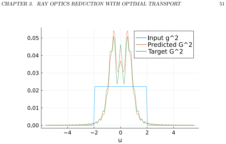
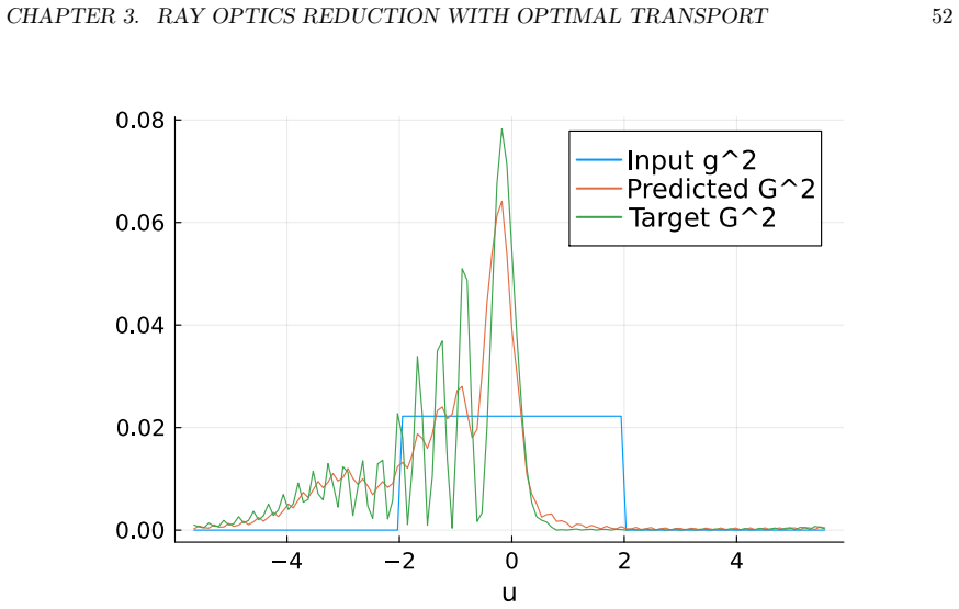
Choose a target phase $\phi(u,v)=\alpha(u^2+v^2)+\beta u^3$ with $\beta$ comparable to $\alpha$, propagate exactly to get $G^2$, run OT initialization followed by Gerchberg-Saxton refinement, and count vortices and measure intensity loss; the paper's Figures 3.8-3.10 already show the loss growing with $\beta$, so a regime where the vortex-free improvement disappears would falsify the claim outside the convex/ray-optics domain.
Extended reading notes
Core claim
The central claim is that the optimal transport plan $\Gamma$ between the squared input intensity $g^2$ and the squared target intensity $G^2$, under quadratic cost, is exactly the zeroth-order stationary-phase term of the Wigner distribution of the unknown field, $W_f^{(0)} = \Gamma$, with $\Gamma(u,\mu)=g(u)^2\delta(\mu-\phi'(u))$ in one dimension. Solving the entropy-regularized OT problem therefore produces a convex, unwrapped phase with no $2\pi$ branch cuts, and using that phase to initialize Gerchberg-Saxton or MRAF eliminates the vortex formation that otherwise stalls convergence. The paper demonstrates numerically that the reconstructed Wigner distribution from the OT-seeded phase matches the ground truth for flat and quadratic phases, and shows how the same reduction applies when the two planes are related by a fractional Fourier transform instead of a plain Fourier transform. On the algorithmic side, writing the Sinkhorn-Knopp updates as Gaussian convolutions reduces the memory cost from $O(n^4)$ to $O(n^2)$ and the runtime from $O(n^4/\epsilon^2)$ to $O(n^2\log n/\epsilon^2)$. The same ray-optics reduction yields a two-shot beam-estimation protocol from two fractional Fourier intensity measurements, and the Hermite-Gaussian expansion of the problem is reinterpreted as a quantum state tomography task.
Load-bearing premise
The load-bearing premise is that the unknown phase is a single smooth, bowl-shaped surface (strictly convex or concave) and that the beam features are large enough relative to focal length and wavelength that diffraction can be neglected; the paper's own cubic-phase simulation shows degraded Wigner estimation and increased intensity loss when a non-convex term is present.
Editorial extensions
If this is right
- OT-initialized Gerchberg-Saxton produces vortex-free phases on smooth targets and reaches an intensity loss roughly an order of magnitude below random or inverse-Fourier initialization, with no efficiency sacrifice.
- Composing OT with MRAF gives a controllable accuracy-efficiency trade-off: near-zero error in a chosen signal region at the cost of a tunable fraction of laser power.
- The convolution form of Sinkhorn-Knopp reduces memory from $O(n^4)$ to $O(n^2)$ and runtime from $O(n^4/\epsilon^2)$ to $O(n^2\log n/\epsilon^2)$, making $1024\times1024$ and larger hologram computations feasible.
- Two diversity images at different fractional Fourier angles are sufficient for a closed OT-based estimate of an unknown beam's amplitude and phase, with error set by the angle separation.
- The same OT/Wigner machinery can retrieve the phase-space (ABCD) transformation of an unknown quadratic-phase optical system from projective intensity measurements.
Reading between the lines
- The identity $W_f^{(0)}=\Gamma$ suggests that the difference $W_\psi-\Gamma$ between the reconstructed Wigner distribution and the transport plan directly measures diffraction and interference corrections, so the norm of that difference could serve as a validity diagnostic for when the ray-optics initialization is trustworthy.
- The convexity limitation suggests a windowed or locally convex extension: decompose a non-convex target into convex patches, solve OT on each patch, and stitch the phases; the paper's cubic-phase experiments indicate exactly where such a scheme would be stress-tested.
- The Hermite-Gaussian/quantum learning formulation implies a concrete algorithmic relaxation not proven in the paper: promote the pure-state vector to a rank-$N$ density matrix in the same constraints, which should make the phase-generation problem feasible even when no pure state exists, at the cost of producing a mixed beam.
Signed reviews
Editorial analysis
A structured set of objections, weighed in public.
Referee Report
Summary. The manuscript presents a ray-optics reduction of phase retrieval. It derives the Monge-Ampere equation from stationary phase, maps that equation to optimal transport, identifies the zero-order term of the Wigner distribution with the OT transport plan, generalizes the argument to fractional Fourier transforms, and uses entropy-regularized OT with a Gaussian-kernel convolution to reduce the memory cost of hologram computation from O(n^4) to O(n^2). The same machinery is applied to beam estimation, and a final chapter sketches a quantum-learning reinterpretation of the phase-generation problem. The text is written as a Stanford BS thesis and includes substantial review material on wave optics, Wigner distributions, and iterative phase-retrieval algorithms.
Significance. If restricted to its demonstrated regime, the paper is a valuable contribution: the stationary-phase derivation of Monge-Ampere, the explicit error parameter beta = 2*pi*R_in*R_out/(f*lambda), and the identification of the OT plan with the zero-order Wigner term are original and pedagogically useful bridges between holography and optimal transport. The O(n^2)-memory Sinkhorn implementation with Gaussian convolutions is a concrete algorithmic improvement over the earlier O(n^4) formulation, and the open-source implementation makes the claims checkable. However, the significance is bounded by the conditions of the theory (strictly convex or concave phase, beta >> 1) and by the fact that the headline performance claims rest on a small number of favorable numerical examples rather than systematic benchmarks. The central theoretical chain is coherent, but the scope of several claims in the abstract and conclusions exceeds what the manuscript proves.
major comments (4)
- [Abstract, Secs. 3.2.3 and 3.4.3] The identity W_f^(0) = Gamma (Eq. 3.58) and the associated vortex-free claim are established only in the ray-optics regime: the stationary-phase reduction assumes a strictly convex or concave phase and beta = 2*pi*R_in*R_out/(f*lambda) >> 1 (Secs. 3.2.2-3.2.3). The paper's own cubic-phase experiment (Eq. 3.72; Figs. 3.8-3.10) shows visibly degraded retrieval and increased intensity loss for a non-convex phase. The abstract, however, presents these results for 'the unknown complex-valued field' without these restrictions. This is a scoping gap rather than an internal inconsistency, but it is load-bearing because the abstract's unconditional phrasing is the headline of the paper; the scope conditions should be stated there and in the conclusions.
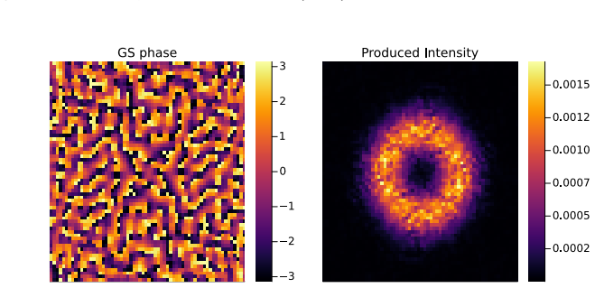
- [Sec. 4.6 and Fig. 4.13] The claim that OT-initialized GS/MRAF yields state-of-the-art accuracy and efficiency and 'completely bypasses' vortex formation is supported by a small set of numerical examples: the Gaussian-to-ring experiment of Sec. 4.2.2 and the 128x128 comparison from [13] reproduced in Fig. 4.13. In Fig. 4.13(j) the MRAF mixing parameter m is hand-tuned to 0.48 to obtain epsilon = 5.95e-16 at 85.15% efficiency, while OT+GS gives 2.58% at 99.91%; this is a favorable demonstration, not a general benchmark. To support the stated generality, the paper should either explicitly restrict the performance claims to smooth, convex, ray-optics-valid targets or provide systematic sweeps over input-output pairs and the two free parameters (epsilon, m).
- [Sec. 3.4.4] The claim in Sec. 3.4.4 and the abstract that the method 'can be used to retrieve the phase-space transformation of any unknown quadratic phase system' is not demonstrated. The section derives only the coefficient A/(2B) for a single collimated input and then states that one or two additional diversity images should suffice, with the 'exact implementations of this idea' left to future work. No full ABCD-matrix retrieval algorithm, numerical experiment, or error analysis is given. This statement should be reframed as a conjecture or the missing construction should be supplied.
- [Sec. 5, Problem 5] The quantum-learning equivalence in Problem 5 is proved only in the infinite-N, zero-error, one-dimensional setting, and the text explicitly concedes that the finite-N, error-tolerant version 'we have not proven it yet.' The abstract's mention of a quantum learning framework and the chapter's framing as a 'deep theoretical connection' therefore outrun the proved content. This secondary claim should be explicitly labeled as a conjecture, or the finite-N proof and the tomographic algorithm with guarantees should be added.
minor comments (5)
- [Theorem 3.2.1] The stationary-phase formula in Eq. (3.14) omits the standard nondegeneracy condition det(nabla^2 psi) != 0; strict convexity alone does not exclude a vanishing Hessian at an isolated point (e.g., x^4), so the theorem's assumptions should be stated precisely.
- [Eq. (3.41)] There is a missing parenthetical grouping in the term 'cot alpha pi (x^2 + y^2)'; it should read pi cot(alpha) (x^2 + y^2) or an equivalent unambiguous expression.
- [Appendix A.5] The text refers to 'Parallel's identity' in Eq. (A.5); this should be 'Parseval's identity.'
- [Sec. 4.2.1] The footnote stating that the convergence conditions were 'summarized from the paper [15] by GPT-o3' is not an appropriate citation style for a scientific article and should be rewritten as a normal scholarly summary with proper attribution.
- [Sec. 4.6] The bullet list in Sec. 4.6 says the method has a single hyperparameter epsilon, but when OT is combined with MRAF, the mixing parameter m is also user-selected, as shown in Fig. 4.13(j); the hyperparameter discussion should acknowledge this coupling.
Circularity Check
No significant circularity: the OT/Wigner identity is a derived mathematical equivalence, not a definitional restatement, and the main claims are tested against ground truth with explicit convexity and ray-optics caveats.
full rationale
The paper's central derivation chain is self-contained. In Sections 3.2.1–3.2.4, the stationary phase approximation is applied to the diffraction integral, and under the stated strict-convexity/concavity assumption it produces the Monge-Ampere equation (3.22). Optimal transport with quadratic cost is then invoked through the standard Brenier theorem (3.24), which gives the same Monge-Ampere equation. This is a derivation, not an assumed equivalence. In Section 3.4.1, the zero-order Wigner approximation W_f^(0) is independently computed by Taylor-expanding the phase and amplitude in the Wigner integral, yielding g^2 δ(φ'-μ). The transport plan Γ for a convex potential satisfying the Monge-Ampere equation has exactly the same form, so Eq. (3.58), W_f^(0)=Γ, is an algebraic identity between two independently defined objects, not a fitted parameter renamed as a prediction. The numerical experiments in Section 3.4.3 compare the retrieved Wigner distribution and propagated intensity against ground truth, and the cubic-phase experiment (Figs. 3.8–3.10) explicitly demonstrates the degradation when the phase is non-convex; this is an honest scoping limitation, not circularity. The abstract's unqualified phrasing is broader than the proven convex case, but that is a scoping gap, not a circular step. Self-citations to [13] are used to identify prior publication of the original algorithm and to point to code and supplementary materials, but the thesis itself contains the derivations and its own numerical validations, with open-source code at [44]. No load-bearing argument reduces to an unverified self-citation, and no external uniqueness theorem is imported from the authors' prior work. The only hyperparameter, ε, is an entropy-regularization parameter, not a quantity fitted to the target and then reported as a prediction. Therefore the paper does not exhibit circular reasoning.
Assumptions & free parameters
free parameters (2)
- entropic regularization epsilon =
1e-3 or 1e-4
- MRAF mixing parameter m =
0.48
assumptions (6)
- standard math Stationary phase approximation for highly oscillatory integrals (Theorem 3.2.1).
- domain assumption Strict convexity or concavity of the unknown phase phi.
- standard math Existence and uniqueness of the Monge-Ampere boundary value problem under mild regularity and convexity assumptions.
- standard math Sinkhorn theorem and generalized Sinkhorn theorem for matrix scaling.
- domain assumption Ray optics validity requires beta = 2*pi*R_in*R_out/(f*lambda) >> 1.
- ad hoc to paper The finite-N quantum learning equivalence (Problem 5) is asserted with only a sketch.
Cite this review
Pith. "Pith review of Ray Optics Approach to Holography." pith.science (2026). https://pith.science/paper/BBYTTI6E
@misc{pith2026250611352,
  author       = {Pith},
  title        = {Pith review of: Ray Optics Approach to Holography},
  year         = {2026},
  howpublished = {\url{https://pith.science/paper/BBYTTI6E}},
  note         = {Machine review of arXiv:2506.11352}
}
read the original abstract
Retrieving the phase of a complex-valued field from the measurements of its amplitude is a crucial problem with a wide range of applications in microscopy and ultracold atomic physics. In particular, obtaining an accurate and efficient solution to this problem is a key step in shaping laser beams for trapping atoms in optical tweezer arrays and applying high-fidelity entangling gates on a neutral atom quantum computer. Current approaches to this problem fail to converge on the optimal solution due to a phenomenon known as vortex formation. In this work, we present an efficient optimization algorithm using Optimal Transport. Our approach completely bypasses the creation of phase vortices and allows for a state-of-the-art solution both in terms of accuracy and efficiency. Furthermore, we show a deep theoretical connection between the Optimal Transport plan and the ray-optics limit of the Wigner distribution of the unknown complex-valued field, and show that our method can be used to retrieve the phase-space transformation of any unknown quadratic phase system. Finally, we reinterpret this problem in the modern quantum learning framework. The techniques we develop provide both useful intuition and practical tools for advancing the frontiers of phase retrieval and laser beam shaping.
Figures


Figures from the paper (43 more)











Reference graph
Works this paper leans on
-
[13]
Van de Graaff, Jan Rudolph, and Jason M
Hunter Swan, Andrii Torchylo, Michael J. Van de Graaff, Jan Rudolph, and Jason M. Hogan. High-fidelity holographic beam shaping with optimal transport and phase diversity, 2024
work page 2024
-
[1]
A high-accuracy algorithm for designing arbitrary holographic atom traps.Opt
Matthew Pasienski and Brian DeMarco. A high-accuracy algorithm for designing arbitrary holographic atom traps.Opt. Express, 16(3):2176–2190, Feb 2008
work page 2008
-
[2]
Georgios Varnavides, Stephanie M. Ribet, Steven E. Zeltmann, Yue Yu, Benjamin H. Savitzky, Dana O. Byrne, Frances I. Allen, Vinayak P. Dravid, Mary C. Scott, and Colin Ophus. Iterative phase retrieval algorithms for scanning transmission electron microscopy, 2024
work page 2024
-
[3]
Liqi Zhou, Jingdong Song, Judy S. Kim, Xudong Pei, Chen Huang, Mark Boyce, Luiza Men- donça, Daniel Clare, Alistair Siebert, Christopher S. Allen, Emanuela Liberti, David Stuart, Xiaoqing Pan, Peter D. Nellist, Peijun Zhang, Angus I. Kirkland, and Peng Wang. Low-dose phase retrieval of biological specimens using cryo-electron ptychography.Nature Communica...
work page 2020
-
[4]
M. D. Barrett, J. A. Sauer, and M. S. Chapman. All-optical formation of an atomic bose-einstein condensate. Phys. Rev. Lett., 87:010404, Jun 2001
work page 2001
-
[5]
Ultracold atomic gases in optical lattices: mimicking condensed matter physics and beyond
Maciej Lewenstein, Anna Sanpera, Veronica Ahufinger, Bogdan Damski, Aditi Sen(De), and Ujjwal Sen. Ultracold atomic gases in optical lattices: mimicking condensed matter physics and beyond. Advances in Physics, 56(2):243–379, 2007
work page 2007
-
[6]
Hogan, Alex Sugarbaker, Susannah M
Tim Kovachy, Jason M. Hogan, Alex Sugarbaker, Susannah M. Dickerson, Christine A. Don- nelly, Chris Overstreet, and Mark A. Kasevich. Matter wave lensing to picokelvin temperatures. Physical Review Letters, 114(14), April 2015
work page 2015
-
[7]
Manetsch, Gyohei Nomura, Elie Bataille, Kon H
Hannah J. Manetsch, Gyohei Nomura, Elie Bataille, Kon H. Leung, Xudong Lv, and Manuel Endres. A tweezer array with 6100 highly coherent atomic qubits, 2024
work page 2024
Show all 61 references
-
[8]
Thompson
Bichen Zhang, Pai Peng, Aditya Paul, and Jeff D. Thompson. Scaled local gate controller for optically addressed qubits.Optica, 11(2):227, February 2024
2024
-
[9]
Zibrov, Manuel Endres, Markus Greiner, Vladan Vuletić, and Mikhail D
Hannes Bernien, Sylvain Schwartz, Alexander Keesling, Harry Levine, Ahmed Omran, Hannes Pichler, Soonwon Choi, Alexander S. Zibrov, Manuel Endres, Markus Greiner, Vladan Vuletić, and Mikhail D. Lukin. Probing many-body dynamics on a 51-atom quantum simulator.Nature, 551(7682):...
2017
-
[10]
Sepehr Ebadi, Tout T. Wang, Harry Levine, Alexander Keesling, Giulia Semeghini, Ahmed Omran, Dolev Bluvstein, Rhine Samajdar, Hannes Pichler, Wen Wei Ho, Soonwon Choi, Subir Sachdev, Markus Greiner, Vladan Vuletić, and Mikhail D. Lukin. Quantum phases of matter on a 256-atom p...
2021
-
[11]
Shaw, Ran Finkelstein, and Manuel Endres
Richard Bing-Shiun Tsai, Xiangkai Sun, Adam L. Shaw, Ran Finkelstein, and Manuel Endres. Benchmarking and fidelity response theory of high-fidelity rydberg entangling gates. PRX Quantum, 6:010331, Feb 2025
2025
-
[12]
Shack-hartmann wavefront sensor optical dynamic range.Opt
Vyas Akondi and Alfredo Dubra. Shack-hartmann wavefront sensor optical dynamic range.Opt. Express, 29(6):8417–8429, Mar 2021
2021
-
[14]
R. W. Gerchberg and W. O. Saxton. A practical algorithm for the determination of plane from image and diffraction pictures.Optik, 35(2):237–246, 1972
1972
-
[15]
Alternating projections with applications to gerchberg-saxton error reduction, 2021
Dominikus Noll. Alternating projections with applications to gerchberg-saxton error reduction, 2021
2021
-
[16]
Bruce, Jonathan Keeling, and Donatella Cassettari
Tiffany Harte, Graham D. Bruce, Jonathan Keeling, and Donatella Cassettari. Conjugate gra- dient minimisation approach to generating holographic traps for ultracold atoms.Opt. Express, 22(22):26548–26558, Nov 2014
2014
-
[17]
Epstein, Leslie Greengard, and Jeremy Magland
Alexander Barnett, Charles L. Epstein, Leslie Greengard, and Jeremy Magland. Geometry of the phase retrieval problem, 2020
2020
-
[18]
Gutiérrez.Optimal Transport and Applications to Geometric Optics
Cristian E. Gutiérrez.Optimal Transport and Applications to Geometric Optics. SpringerBriefs on PDEs and Data Science. Springer Singapore, 1 edition, 2023
2023
-
[19]
Light in power: a general and parameter- free algorithm for caustic design.ACM Transactions on Graphics (TOG), 37(6):1–13, 2018
Jocelyn Meyron, Quentin Mérigot, and Boris Thibert. Light in power: a general and parameter- free algorithm for caustic design.ACM Transactions on Graphics (TOG), 37(6):1–13, 2018
2018
-
[20]
Optical design of single reflector systems and the monge– kantorovich mass transfer problem.Journal of Mathematical Sciences, 117(3):4096–4108, 2003
Tilmann Glimm and Vladimir Oliker. Optical design of single reflector systems and the monge– kantorovich mass transfer problem.Journal of Mathematical Sciences, 117(3):4096–4108, 2003
2003
-
[21]
On the design of a reflector antenna II
Xu-Jia Wang. On the design of a reflector antenna II. Calculus of Variations and Partial Differential Equations, 20(3):329–341, 2004
2004
-
[22]
High-contrast computational caustic design.ACM Transactions on Graphics (TOG), 33(4):1–11, 2014
Yuliy Schwartzburg, Romain Testuz, Andrea Tagliasacchi, and Mark Pauly. High-contrast computational caustic design.ACM Transactions on Graphics (TOG), 33(4):1–11, 2014
2014
-
[23]
The Refractor Problem in Reshaping Light Beams
Cristian E Gutiérrez and Qingbo Huang. The Refractor Problem in Reshaping Light Beams. Arch. Ration. Mech. Anal., 193(2):423–443, 2009
2009
-
[24]
Dickey.Laser Beam Shaping: Theory and Techniques
Fred M. Dickey.Laser Beam Shaping: Theory and Techniques. CRC Press, Boca Raton, FL, 2nd edition, 2014. BIBLIOGRAPHY 138
2014
-
[25]
Murat Ozaktas, M
H. Murat Ozaktas, M. Alper Kutay, and Zeev Zalevsky.The Fractional Fourier Transform with Applications in Optics and Signal Processing. Wiley, 2001
2001
-
[26]
A.E. Siegman. Lasers. G - Reference,Information and Interdisciplinary Subjects Series. Uni- versity Science Books, 1986
1986
-
[27]
Young.An Introduction to Hilbert Space
N. Young.An Introduction to Hilbert Space. Cambridge University Press, 1988
1988
-
[28]
Laguerre–gaussian modes and the wigner transform
Michael VanValkenburgh. Laguerre–gaussian modes and the wigner transform. Journal of Modern Optics, 55(21):3537–3549, December 2008
2008
-
[29]
Psycharakis, Evangelos Liapis, Jorge Ripoll, and Giannis Zacharakis
Daniele Ancora, Diego Di Battista, Georgia Giasafaki, Stylianos E. Psycharakis, Evangelos Liapis, Jorge Ripoll, and Giannis Zacharakis. Optical projection tomography via phase retrieval algorithms. Methods, 136:81–89, 2018. Methods in Quantitative Phase Imaging in Life Science
2018
-
[30]
Handelsman
Norman Bleistein and Richard A. Handelsman. Asymptotic Expansions of Integrals. Dover Publications, New York, corrected dover reprint of the 1975 original edition, 1986. See Chap.8, §8.4, eq.(8.4.10) for the 2-D stationary-phase formula
1975
-
[31]
Caffarelli
Luis A. Caffarelli. Interiorw2,p estimates for solutions of the monge–ampère equation.Annals of Mathematics, 131(1):135–150, 1990
1990
-
[32]
On the second boundary value problem for equations of monge–ampère type
John Urbas. On the second boundary value problem for equations of monge–ampère type. Journal für die reine und angewandte Mathematik, 487:115–124, 1997
1997
-
[33]
Optimaltransport.jl
Tim Matsumoto, David Widmann, Davi Barreira, and Stephen Zhang. Optimaltransport.jl. https://github.com/JuliaOptimalTransport/OptimalTransport.jl, commit: 9da044c, 2022
2022
-
[34]
Pot: Python optimal transport.The Journal of Machine Learning Research, 22(1):3571–3578, 2021
Rémi Flamary, Nicolas Courty, Alexandre Gramfort, Mokhtar Z Alaya, Aurélie Boisbunon, Stanislas Chambon, Laetitia Chapel, Adrien Corenflos, Kilian Fatras, Nemo Fournier, et al. Pot: Python optimal transport.The Journal of Machine Learning Research, 22(1):3571–3578, 2021
2021
-
[35]
Optimal Transport: Old and New, volume 338
Cédric Villani. Optimal Transport: Old and New, volume 338. Springer, 2009
2009
-
[36]
Topics in optimal transportation, volume 58
Cédric Villani. Topics in optimal transportation, volume 58. American Mathematical Soc., 2021
2021
-
[37]
Décomposition polaire et réarrangement monotone des champs de vecteurs.CR Acad
Yann Brenier. Décomposition polaire et réarrangement monotone des champs de vecteurs.CR Acad. Sci. Paris Sér. I Math., 305:805–808, 1987
1987
-
[38]
Polar factorization and monotone rearrangement of vector-valued functions
Yann Brenier. Polar factorization and monotone rearrangement of vector-valued functions. Communications on Pure and Applied Mathematics, 44(4):375–417, 1991
1991
-
[39]
The Monge–Ampère equation and its link to optimal transportation
Guido De Philippis and Alessio Figalli. The Monge–Ampère equation and its link to optimal transportation. Bulletin of the American Mathematical Society, 51(4):527–580, 2014. BIBLIOGRAPHY 139
2014
-
[40]
Goldstein
Ward Cheney and Allen A. Goldstein. Proximity maps for convex sets. Proceedings of the American Mathematical Society, 10(3):448–450, 1959
1959
-
[41]
Bijnen, van.Quantum engineering with ultracold atoms
R.M.W. Bijnen, van.Quantum engineering with ultracold atoms. Phd thesis 1 (research tu/e / graduation tu/e), Applied Physics and Science Education, 2013
2013
-
[42]
Kaiqiang Wang, Li Song, Chutian Wang, Zhenbo Ren, Guangyuan Zhao, Jiazhen Dou, Jianglei Di, George Barbastathis, Renjie Zhou, Jianlin Zhao, and Edmund Y. Lam. On the use of deep learning for phase recovery.Light: Science & Applications, 13(1), January 2024
2024
-
[43]
Phase imaging with an untrained neural network
Fei Wang, Yaoming Bian, Haichao Wang, Meng Lyu, Giancarlo Pedrini, Wolfgang Osten, George Barbastathis, and Guohai Situ. Phase imaging with an untrained neural network. Light: Science & Applications, 9(1):77, May 2020
2020
-
[44]
SLMTools.https://github.com/ hoganphysics/SLMTools, commit: d7db9fd, 2024
Hunter Swan, Michael Van de Graaff, and Andrii Torchylo. SLMTools.https://github.com/ hoganphysics/SLMTools, commit: d7db9fd, 2024
2024
-
[45]
Computational optimal transport, 2020
Gabriel Peyré and Marco Cuturi. Computational optimal transport, 2020
2020
-
[46]
Cambridge University Press, 2004
Stephen Boyd and Lieven Vandenberghe.Convex Optimization. Cambridge University Press, 2004
2004
-
[47]
Sinkhorndistances: Lightspeedcomputationofoptimaltransportationdistances, 2013
MarcoCuturi. Sinkhorndistances: Lightspeedcomputationofoptimaltransportationdistances, 2013
2013
-
[48]
A Relationship Between Arbitrary Positive Matrices and Doubly Stochastic Matrices
Richard Sinkhorn. A Relationship Between Arbitrary Positive Matrices and Doubly Stochastic Matrices. The Annals of Mathematical Statistics, 35(2):876 – 879, 1964
1964
-
[49]
On sinkhorn’s representation of nonnegative matrices.Journal of Mathematical Analysis and Applications, 54(3):674–677, 1976
Helge Tverberg. On sinkhorn’s representation of nonnegative matrices.Journal of Mathematical Analysis and Applications, 54(3):674–677, 1976
1976
-
[50]
A review of matrix scaling and sinkhorn’s normal form for matrices and positive maps, 2016
Martin Idel. A review of matrix scaling and sinkhorn’s normal form for matrices and positive maps, 2016
2016
-
[51]
Computational optimal trans- port: Complexity by accelerated gradient descent is better than by sinkhorn’s algorithm, 2018
Pavel Dvurechensky, Alexander Gasnikov, and Alexey Kroshnin. Computational optimal trans- port: Complexity by accelerated gradient descent is better than by sinkhorn’s algorithm, 2018
2018
-
[52]
Stabilized sparse scaling algorithms for entropy-regularized transport problems
Bernhard Schmitzer. Stabilized sparse scaling algorithms for entropy-regularized transport problems. SIAM Journal on Scientific Computing, 41(3):A1443–A1481, 2019
2019
-
[53]
Overrelaxed sinkhorn– knopp algorithm for regularized optimal transport.arXiv preprint, 2017
Alexis Thibault, Lénaïc Chizat, Charles Dossal, and Nicolas Papadakis. Overrelaxed sinkhorn– knopp algorithm for regularized optimal transport.arXiv preprint, 2017. v2, March 2021
2017
-
[54]
Robert J. Berman. The sinkhorn algorithm, parabolic optimal transport and geometric monge– ampère equations. Numerische Mathematik, 145(4):771–836, 2020. BIBLIOGRAPHY 140
2020
-
[55]
Rethinking initialization of the sinkhorn algorithm
James Thornton and Marco Cuturi. Rethinking initialization of the sinkhorn algorithm. In Proc. 26th Int. Conf. on Artificial Intelligence and Statistics (AISTATS), pages 7728–7754. PMLR, 2023
2023
-
[56]
A Survey of Gaussian Convolution Algorithms.Image Processing On Line, 3:286–310, 2013
Pascal Getreuer. A Survey of Gaussian Convolution Algorithms.Image Processing On Line, 3:286–310, 2013. https://doi.org/10.5201/ipol.2013.87
2013 doi
-
[57]
Kick-off seminar — optimal transport, statistics and learning
Gabriel Peyré. Kick-off seminar — optimal transport, statistics and learning. https: //kantorovich.org/event/kickoff_peyre/, 2023. Accessed: 2025-05-15
2023
-
[58]
Andrews, Richard Askey, and Ranjan Roy.Special Functions, volume 71 ofEncyclo- pedia of Mathematics and its Applications
George E. Andrews, Richard Askey, and Ranjan Roy.Special Functions, volume 71 ofEncyclo- pedia of Mathematics and its Applications. Cambridge University Press, Cambridge, 1999
1999
-
[59]
Madalin Guta, Jonas Kahn, Richard Kueng, and Joel A. Tropp. Fast state tomography with optimal error bounds, 2018
2018
-
[60]
Santhanam
Balu Santhanam and Thalanayar S. Santhanam. Discrete gauss-hermite functions and eigen- vectors of the centered discrete fourier transform. In2007 IEEE International Conference on Acoustics, Speech and Signal Processing - ICASSP ’07, volume 3, pages III–1385–III–1388, 2007
2007
-
[61]
Claasen and W
T. Claasen and W. Mecklenbrauker. The aliasing problem in discrete-time wigner distributions. IEEE Transactions on Acoustics, Speech, and Signal Processing, 31(5):1067–1072, 1983
1983
Reviewed August 7, 2026 · model on record in the stance chip above.
Discussion (0). Continue with ORCID to comment.