REVIEW 1 major objections 6 minor 30 references
Data-driven approaches to inverse problems
T0 review · 1 major / 6 minor · reviewed 2026-08-07 · deepseek-v4-flash
Pith's one-line read These lecture notes argue that data-driven solvers for inverse problems can be both highly accurate and mathematically trustworthy when learned components are embedded in classical variational regularization, through mechanisms such as…
desk verdict Useful lecture notes on data-driven inverse problems, but Theorem 3.2.4 misstates the distance function and should be corrected before the notes are used as a reference. read the letter →
The pith
A machine-rendered reading of the paper's core claim, the machinery that carries it, and where it could break.
The reading
What carries the argument
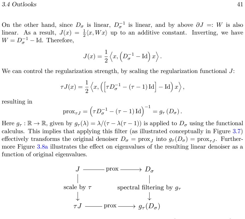
The load-bearing object is the proximal operator of convex analysis, $\mathrm{prox}_J=(I+\partial J)^{-1}$, because it is the bridge between variational regularization and denoisers: a plug-and-play scheme replaces the proximal step of a regularizer by a denoiser. For a linear denoiser $D_\sigma$, the notes use the equivalence $J(x)=\frac{1}{2}\langle x,(D_\sigma^{-1}-I)x\rangle$ and derive that scaling $J$ by $\tau$ corresponds to the spectral filter $g_\tau(\lambda)=\lambda/(\tau-\lambda(\tau-1))$ applied to the eigenvalues of $D_\sigma$, so $\mathrm{prox}_{\tau J}=g_\tau(D_\sigma)$. That identity converts a fixed denoiser into a one-parameter family of regularization operators and makes the convergence-to-truth result possible. On the adversarial side, the key object is a regularizer $R_\Theta(u)=\Psi_\Theta(u)+\rho_0|u|^2/2$ trained through a Wasserstein-1 loss with a gradient penalty; its role is to encode the geometry of the clean-image distribution without paired supervision, with the distance to the data manifold serving as the ideal regularizer under the stated assumptions.
What would settle it
Take a trained deep denoiser and compute its Jacobian at several natural images: if the Jacobian is not symmetric with eigenvalues in $[0,1]$, the denoiser cannot be the proximal operator of a convex functional, and the spectral-filtering convergence theorem in the notes does not cover it. Alternatively, run the filtered plug-and-play iteration on a known ground-truth case with noise levels $\delta\to 0$: if reconstruction error does not approach zero under the prescribed parameter rule, the claimed convergent-regularization property fails.
Extended reading notes
Core claim
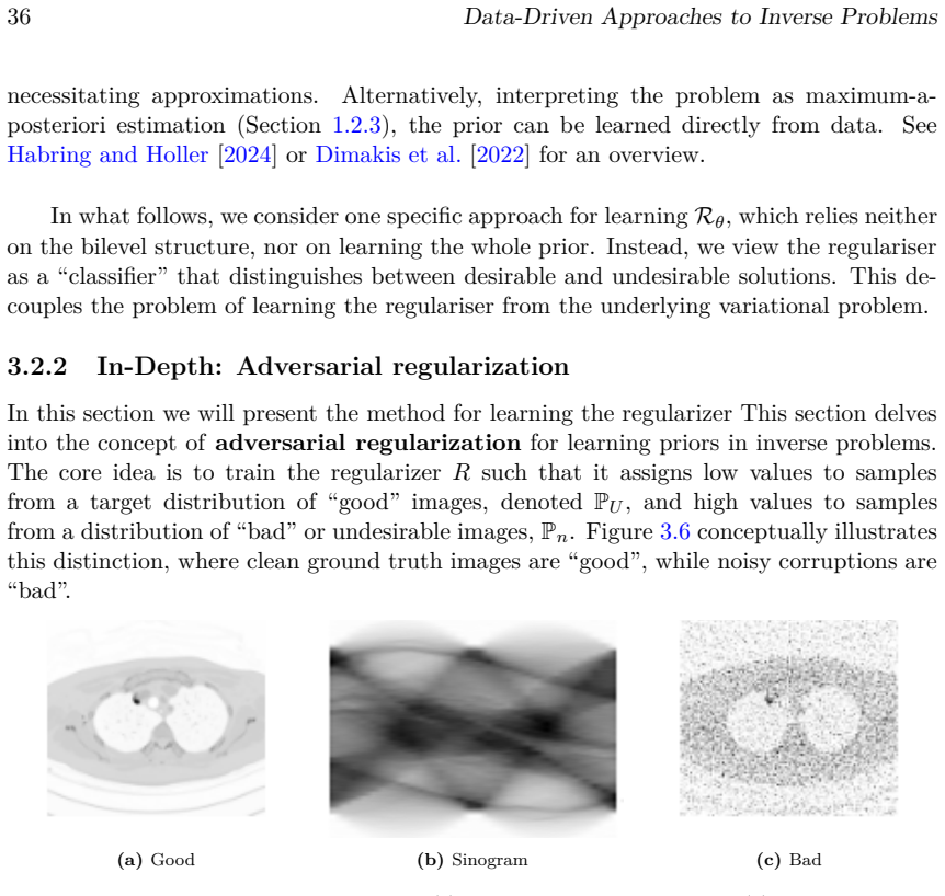
On the paper's terms, the central discovery is that the dichotomy between mathematical reconstruction and deep learning is false: learned components can be grafted onto the variational formulation $\min_u D(Au,y)+\alpha R(u)$ and still inherit its stability and convergence. Adversarial regularization trains $R$ as a 1-Lipschitz function that assigns low values to clean images and high values to corrupted ones, using a Wasserstein-1 loss that does not require paired examples; under a data-manifold and low-noise assumption, the distance to the data manifold is a maximizer of that loss, and the gradient flow of the trained regularizer decreases the Wasserstein distance at the fastest possible rate. For plug-and-play methods, the notes show that when a linear denoiser is symmetric and positive semi-definite with eigenvalues in $[0,1]$, it is the proximal operator of a convex functional $J$, and scaling $J$ by $\tau$ is implemented by filtering the denoiser's eigenvalues through $g_\tau(\lambda)=\lambda/(\tau-\lambda(\tau-1))$; with a suitable parameter rule this gives a convergent regularization, a guarantee absent from generic learned iterative schemes. The notes also argue that unconstrained fully learned methods can hallucinate structures in severely ill-posed problems even when their pixel metrics improve, so mathematical structure is not an optional extra but the condition for reliability.
Load-bearing premise
The convergent plug-and-play guarantee rests on the assumption that the denoiser is linear, symmetric, and positive semi-definite, meaning it is exactly the proximal map of some convex penalty; because trained deep denoisers are neither linear nor symmetric, the guarantee does not directly cover them.
Editorial extensions
If this is right
- Learned regularizers trained with a Wasserstein separation loss can be inserted into variational problems and inherit existence, uniqueness, stability, and convergence guarantees from the classical theory.
- A linear plug-and-play denoiser whose eigenvalues are filtered by $g_\tau$ defines a convergent regularization: as the noise level $\delta$ tends to zero and $\tau$ is chosen by a suitable rule, the reconstruction converges to the underlying solution.
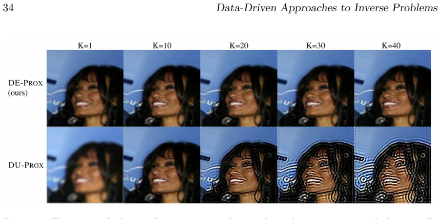
- Deep equilibrium networks that constrain the learned update to be a contraction converge to a fixed point even beyond the number of training steps, avoiding the divergence artifacts seen in unconstrained unrolled networks.
- Jointly training reconstruction and a downstream task such as segmentation can improve the downstream task relative to isolated training, because the extra degrees of freedom of an ill-posed problem can be steered toward task-relevant reconstructions.
- Purely learned methods can report better PSNR and SSIM while hallucinating anatomical structures in severely ill-posed problems, so reliability requires grounding learned components in mathematical guarantees.
Reading between the lines
- Editorial inference: if the spectral-filtering construction can be extended to nonlinear denoisers, for instance through the Tweedie-scaling ideas the notes cite, then pretrained deep denoisers could be endowed with convergent-regularization guarantees without being retrained under restrictive linearity constraints.
- Editorial inference: the data-manifold characterization of adversarial regularizers suggests a natural out-of-distribution detector, since images with unusually high regularizer values sit far from the learned clean distribution, which could support uncertainty quantification in clinical deployment.
- Editorial inference: the same eigenvalue-filtering logic gives a principled calibration rule for regularization strength in other operator-splitting schemes beyond plug-and-play, potentially replacing heuristics such as denoiser scaling with a parameter rule that has a convergence guarantee.
- Editorial inference: task-adapted reconstruction implies that evaluation benchmarks for imaging should weight downstream diagnostic utility at least as heavily as pixel-level metrics, since a reconstruction can be better for segmentation without having better PSNR.
Editorial analysis
A structured set of objections, weighed in public.
Referee Report
Summary. These lecture notes provide an introduction to inverse problems and survey both classical and data-driven reconstruction approaches. The first part covers well-posedness, variational regularization, total variation and PDE-based methods, and the main numerical optimization tools. The second part discusses learned iterative schemes, learned variational models with a focus on adversarial regularization, and plug-and-play methods, including a spectral-filtering construction for linear denoisers that yields convergent regularization. The notes argue that combining deep learning with rigorous regularization theory is necessary for reliable and interpretable reconstruction, and they close with perspectives on task adaptation and open problems.
Significance. The notes are a valuable and readable survey of an active area, with the considerable strength that they consistently separate provable results from empirical heuristics. The discussion of learned iterative schemes honestly documents their lack of convergence guarantees and the risk of hallucination in severely ill-posed problems, and the spectral-filtering treatment of linear plug-and-play denoisers gives a concrete, parameter-free mechanism for controlling regularization strength. The authors also give useful pointers to their own convergence results for weakly convex regularizers. However, the theoretical justification of adversarial regularization contains a genuine mathematical error in Theorem 3.2.4, and this must be corrected before the notes can serve as a reliable reference.
major comments (1)
- [§3.2.2, Theorem 3.2.4] The theorem states that, under the Data Manifold Assumption and the Low Noise Assumption, the squared distance function u ↦ min_{v∈M} ‖u−v‖² is a maximizer of the Wasserstein loss (3.5) over all 1-Lipschitz functions R. This is not correct as stated: on Rⁿ the squared distance has gradient 2(u−P_M(u)), whose norm is unbounded when the domain is unbounded, so it is not 1-Lipschitz and is therefore not admissible in the supremum defining (3.5). The assumptions DMA and LNA do not restrict the support of the noisy distribution P_n to a bounded set, so the classical remedy of restricting to a compact domain does not apply. The correct and standard statement uses the unsquared distance d_M(u)=min_{v∈M} ‖u−v‖, which is 1-Lipschitz. Because Theorem 3.2.4 is the explicit theoretical justification for adversarial regularization advertised in the abstract, the statement must be corrected or replaced with the correct theorem, with a precise citation to the original source.
minor comments (6)
- [§1.2.1, Definition 1.2.1] The definition says 'R_α y → A†y = u† for all f ∈ dom(A†)'; the quantifier should be 'for all y ∈ dom(A†)', not 'for all f'.
- [§1.2.2, Theorem 1.2.2] The last line of the theorem statement says 'generalizing Theorem 1.2.1', but there is no Theorem 1.2.1; the intended cross-reference is likely Definition 1.2.1. Also, the proof is only referenced to Mukherjee et al. [2024], which is acceptable for lecture notes, but the reference should be made explicit in the statement.
- [§1.1, Example 1.1.2] The dimensions are used inconsistently: the first bullet writes 'n < m' for A: Rⁿ → ran(A) ⊂ Rᵐ, while the second bullet writes 'n > m and A: Rᵈ → Rᵐ' with an undefined symbol d; this should be A: Rⁿ → Rᵐ.
- [§2.4, Examples 2.4.1 and surrounding text] The text refers to 'Theorem 2.4.1' and Example 2.4.1 refers to 'Theorem 2.3.1', but neither theorem exists; these should be cross-references to the named ROF problem or to the appropriate example/definition numbers.
- [§3.3.2, Figure 3.8] The text defines the spectral filter as g_τ(λ)=λ/(τ−λ(τ−1)), but the vertical axis of Figure 3.8a is labeled 'h_τ(λ)'; the notation should be made consistent.
- [§3.3.2] The assumptions that the linear denoiser is symmetric, positive semi-definite, non-expansive, and has bounded inverse are stated in prose; since they are the crucial hypotheses for the convergent-regularization result, they should be displayed as a formal assumption and followed by an explicit remark that most learned deep denoisers do not satisfy them, so the result does not directly apply in the general nonlinear setting.
Circularity Check
No significant circularity: the notes are a survey whose load-bearing results are external theorems or explicit derivations, and the self-citations are not used as circular premises.
full rationale
The paper is a lecture-note survey rather than a derivation of a single new prediction. Its main mathematical ingredients are textbook or external results: Tikhonov well-posedness, TV regularization, convex analysis, PDHG, and the cited theorems in Sections 3.1.2, 3.2.2, and 3.3.2 are stated with assumptions and proofs located in the cited literature, not manufactured inside the notes. Section 3.3.2 explicitly derives the quadratic functional J(x) = (1/2)<x,(D_sigma^{-1}-Id)x> from the proximal-operator identity and linearity of D_sigma, then constructs the spectral filter g_tau; no fitted parameter is renamed as a prediction. Several cited works are co-authored by the present authors (e.g., Mukherjee et al. 2023, Shumaylov et al. 2024, Hauptmann et al. 2024), but these citations provide context, convergence theorems, and empirical illustrations; they are not the sole justification of a claim whose content reduces to the citation itself. The Wasserstein-loss maximizer statement in Theorem 3.2.4 is questionable as written because the squared distance function is not 1-Lipschitz on unbounded domains; however, that is a correctness concern, not a circularity, and does not affect the circularity score. No step was found in which the conclusion is equivalent to an input by definition or in which a fitted quantity is presented as a prediction.
Assumptions & free parameters
assumptions (4)
- standard math Standard results in functional analysis and convex analysis (e.g., subdifferentials, Legendre-Fenchel duality) are used throughout.
- domain assumption The noise model is additive and bounded as in Equation (1.1).
- domain assumption Cited theorems (e.g., Theorem 3.1.1 from Gilton et al., Theorem 3.2.1 from Lunz et al., Theorem 3.2.4) are correct as stated.
- domain assumption The Data Manifold Assumption and Low Noise Assumption in Section 3.2.2 hold.
Cite this review
Pith. "Pith review of Data-driven approaches to inverse problems." pith.science (2026). https://pith.science/paper/UF2QJ4QV
@misc{pith2026250611732,
  author       = {Pith},
  title        = {Pith review of: Data-driven approaches to inverse problems},
  year         = {2026},
  howpublished = {\url{https://pith.science/paper/UF2QJ4QV}},
  note         = {Machine review of arXiv:2506.11732}
}
read the original abstract
Inverse problems are concerned with the reconstruction of unknown physical quantities using indirect measurements and are fundamental across diverse fields such as medical imaging, remote sensing, and material sciences. These problems serve as critical tools for visualizing internal structures beyond what is visible to the naked eye, enabling quantification, diagnosis, prediction, and discovery. However, most inverse problems are ill-posed, necessitating robust mathematical treatment to yield meaningful solutions. While classical approaches provide mathematically rigorous and computationally stable solutions, they are constrained by the ability to accurately model solution properties and implement them efficiently. A more recent paradigm considers deriving solutions to inverse problems in a data-driven manner. Instead of relying on classical mathematical modeling, this approach utilizes highly over-parameterized models, typically deep neural networks, which are adapted to specific inverse problems using carefully selected training data. Current approaches that follow this new paradigm distinguish themselves through solution accuracy paired with computational efficiency that was previously inconceivable. These notes offer an introduction to this data-driven paradigm for inverse problems. The first part of these notes will provide an introduction to inverse problems, discuss classical solution strategies, and present some applications. The second part will delve into modern data-driven approaches, with a particular focus on adversarial regularization and provably convergent linear plug-and-play denoisers. Throughout the presentation of these methodologies, their theoretical properties will be discussed, and numerical examples will be provided. The lecture series will conclude with a discussion of open problems and future perspectives in the field.
Figures


Figures from the paper (19 more)




Reference graph
Works this paper leans on
-
[9]
S. Hurault, A. Leclaire, and N. Papadakis. Gradient step denoiser for convergent plug- and-play.arXiv preprint arXiv:2110.03220,
-
[21]
M. L. Saksman, S. Siltanen, et al. Discretization-invariant bayesian inversion and besov space priors.arXiv preprint arXiv:0901.4220,
-
[22]
P. Sellars, A. I. Aviles-Rivero, N. Papadakis, D. Coomes, A. Faul, and C.-B. Schönlieb. Semi-supervised learning with graphs: Covariance based superpixels for hyperspectral image classification. InIGARSS 2019-2019 IEEE International Geoscience and Remote Sensing Symposium, pages 592–595. IEEE,
work page 2019
-
[23]
Z. Shumaylov, J. Budd, S. Mukherjee, and C.-B. Schönlieb. Provably convergent data- driven convex-nonconvex regularization. InNeurIPS 2023 Workshop on Deep Learning and Inverse Problems,
work page 2023
-
[24]
URL https://openreview.net/forum?id=7PLpiVdnUC. J. Stanczuk, C. Etmann, L. M. Kreusser, and C.-B. Schönlieb. Wasserstein gans work because they fail (to approximate the wasserstein distance).arXiv preprint arXiv:2103.01678,
-
[26]
H. Y. Tan, Z. Cai, M. Pereyra, S. Mukherjee, J. Tang, and C.-B. Schönlieb. Unsupervised training of convex regularizers using maximum likelihood estimation.Transactions on Machine Learning Research, 2024a. H. Y. Tan, S. Mukherjee, J. Tang, and C.-B. Schönlieb. Provably convergent plug-and-play quasi-newton methods.SIAM Journal on Imaging Sciences, 17(2):7...
-
[27]
J. Tang, S. Mukherjee, and C.-B. Schönlieb. Iterative operator sketching framework for large-scale imaging inverse problems. InICASSP 2025-2025 IEEE International Con- ference on Acoustics, Speech and Signal Processing (ICASSP), pages 1–5. IEEE,
work page 2025
- [28]
Show all 30 references
-
[30]
URLhttps://arxiv.org/abs/2002.11546
2002 arXiv
-
[1965]
Moreau and J
T. Moreau and J. Bruna. Understanding trainable sparse coding via matrix factorization. arXiv preprint arXiv:1609.00285,
-
[1992]
Rudzusika, B
J. Rudzusika, B. Bajić, O. Öktem, C.-B. Schönlieb, and C. Etmann. Invertible learned primal-dual. InNeurIPS 2021 Workshop on Deep Learning and Inverse Problems, on- line,
2021
-
[1993]
Masnou and J.-M
S. Masnou and J.-M. Morel. Level lines based disocclusion. InProceedings 1998 Interna- tional Conference on Image Processing. ICIP98 (Cat. No. 98CB36269), pages 259–263. IEEE,
1998
-
[1998]
Staudt, S
T. Staudt, S. Hundrieser, and A. Munk. On the uniqueness of Kantorovich potentials. arXiv preprint arXiv:2201.08316,
-
[2001]
Novaga and E
M. Novaga and E. Paolini. Regularity results for boundaries in r2 with prescribed anisotropic curvature.Annali di Matematica Pura ed Applicata (1923-), 2(184):239– 261,
1923
-
[2004]
De Giorgi
E. De Giorgi. Variational free-discontinuity problems. InInternational Conference in Memory of Vito Volterra (Italian) (Rome, 1990), volume 92 ofAtti Convegni Lincei, pages 133–150. Accad. Naz. Lincei, Rome,
1990
-
[2005]
Obmann and M
D. Obmann and M. Haltmeier. Convergence analysis of equilibrium methods for inverse problems.arXiv preprint arXiv:2306.01421,
-
[2008]
Putzky and M
P. Putzky and M. Welling. Recurrent inference machines for solving inverse problems. arXiv preprint arXiv:1706.04008,
-
[2009]
URLhttps://doi.org/10.1137/080728548
doi: 10.1137/080728548. URLhttps://doi.org/10.1137/080728548. X. Cai, R. Chan, and T. Zeng. A two-stage image segmentation method using a con- vex variant of the mumford–shah model and thresholding.SIAM Journal on Imaging Sciences, 6(1):368–390,
-
[2010]
Buades, B
A. Buades, B. Coll, and J.-M. Morel. A non-local algorithm for image denoising. In 2005 IEEE computer society conference on computer vision and pattern recognition (CVPR’05), volume 2, pages 60–65. Ieee,
2005
-
[2012]
D. Wu, K. Kim, B. Dong, G. E. Fakhri, and Q. Li. End-to-end lung nodule detection in computed tomography. InMachine Learning in Medical Imaging: 9th International Workshop, MLMI 2018, Held in Conjunction with MICCAI 2018, Granada, Spain, September 16, 2018, Proceedings 9, page...
2018
-
[2014]
J. M. Borwein and D. R. Luke. Duality and convex programming.Handbook of Mathe- matical Methods in Imaging, 2015:257–304,
2015
-
[2016]
Mukherjee, C.-B
S. Mukherjee, C.-B. Schönlieb, and M. Burger. Learning convex regularizers satisfying the variational source condition for inverse problems.arXiv preprint arXiv:2110.12520,
-
[2017]
Milne, Étienne Bilocq, and A
T. Milne, Étienne Bilocq, and A. Nachman. A new method for determining Wasserstein 1 optimal transport maps from Kantorovich potentials, with deep learning applications. arXiv preprint arXiv:2211.00820,
-
[2018]
A. I. Aviles-Rivero, N. Papadakis, R. Li, P. Sellars, Q. Fan, R. T. Tan, and C.-B. Schönlieb. Graphxˆ\small net-net-chest x-ray classification under extreme minimal supervision. In Medical Image Computing and Computer Assisted Intervention–MICCAI 2019: 22nd International Confe...
2019
-
[2019]
Gilton, G
D. Gilton, G. Ongie, and R. Willett. Deep equilibrium architectures for inverse problems in imaging.IEEE Transactions on Computational Imaging, 7:1123–1133, 2021a. D. Gilton, G. Ongie, and R. Willett. Model adaptation for inverse problems in imaging. IEEE Transactions on Compu...
2016
-
[2020]
Driggs, J
4.2 The Data Driven - Knowledge Informed Paradigm55 D. Driggs, J. Tang, J. Liang, M. Davies, and C.-B. Schonlieb. A stochastic proximal alternating minimization for nonsmooth and nonconvex optimization.SIAM Journal on Imaging Sciences, 14(4):1932–1970,
1932
-
[2021]
Khelifa, F
58Perspectives N. Khelifa, F. Sherry, and C.-B. Schönlieb. Enhanced denoising and convergent regulari- sation using tweedie scaling.arXiv preprint arXiv:2503.05956,
-
[2023]
2022.3207451
doi: 10.1109/MSP. 2022.3207451. URLhttps://ieeexplore.ieee.org/abstract/document/10004773. S. Mukherjee, S. Dittmer, Z. Shumaylov, S. Lunz, O. Öktem, and C.-B. Schönlieb. Data- driven convex regularizers for inverse problems. InICASSP 2024-2024 IEEE Interna- tional Conference ...
2022
-
[2024]
A. Hertle. On the problem of well-posedness for the radon transform. InMathematical Aspects of Computerized Tomography: Proceedings, Oberwolfach, February 10–16, 1980, pages 36–44. Springer,
1980
-
[2025]
URLhttps://www.aimsciences.org/article/ id/67ab0b783942fc6603063e6e
doi: 10.3934/ammc.2025001. URLhttps://www.aimsciences.org/article/ id/67ab0b783942fc6603063e6e. E. Kobler, T. Klatzer, K. Hammernik, and T. Pock. Variational networks: connecting variational methods and deep learning. InPattern Recognition: 39th German Confer- ence, GCPR 2017,...
Reviewed August 7, 2026 · model on record in the stance chip above.
Discussion (0). Continue with ORCID to comment.