REVIEW 4 major objections 6 minor 58 references
CLGNN: A Contrastive Learning-based GNN Model for Betweenness Centrality Prediction on Temporal Graphs
T0 review · 4 major / 6 minor · reviewed 2026-08-07 · deepseek-v4-flash
Pith's one-line read CLGNN predicts temporal betweenness centrality with up to 31.4x lower MAE than static GNNs and up to 5.7x lower than temporal GNNs, while running up to 663.7x faster than exact computation.
desk verdict A plausible new model for temporal betweenness prediction whose reported gains are undermined by an underspecified evaluation protocol; worth reviewing carefully, not desk-rejecting. read the letter →
The pith
A machine-rendered reading of the paper's core claim, the machinery that carries it, and where it could break.
The reading
What carries the argument
The load-bearing objects are the temporal path-count encoding and the clustering-guided contrastive loss. For each directed interaction $(u,v,t)$, the count $P(u,v,t)=\sum_{t_v \in T_{\text{out}}(v)} I(t_v - t)$ records how many outgoing temporal edges from $v$ can continue the path within the time budget; this scalar, log-transformed and MLP-encoded, tells the network which messages are on valid time-respecting paths and gates message passing. The second mechanism, KContrastNet, first selects the number of clusters $\hat{k}$ by minimizing bootstrap K-means instability, then builds positive pairs from same-cluster nodes with similar TBC and negative pairs from same-cluster nodes with very different TBC, with weights $\beta_{uv}$ inversely or directly proportional to TBC difference. This forces the representation space to separate zero-, median-, and high-centrality nodes while keeping the regression module stable.
What would settle it
Train CLGNN and its baselines on a fully specified held-out protocol — the 50 training networks named, the 12 evaluation networks never seen in training, and learning rates selected on a validation split — then check whether CLGNN's MAE advantage over DBGNN and TGAT persists at the reported 5.7x and 9.4x margins; if the margins shrink to near parity under that protocol, the central claim fails.
Extended reading notes
Core claim
The central claim is that pairwise contrastive supervision over cluster-structured node embeddings, guided by the TBC distribution itself, lets a temporal GNN regress TBC values without being swamped by the zero-value majority. Concretely, CLGNN encodes each interaction with a message that concatenates previous-layer node states, a continuous-time encoding, and a temporal path count $P(u,v,t)$ that counts how many valid temporal continuations exist after edge $(u,v,t)$; a dual aggregator combines mean neighbor messages with edge-to-node multi-head attention. A stability-based clustering module estimates the number of TBC-consistent clusters via bootstrap resampling and K-means, and the KContrastNet loss pulls together nodes in the same cluster with similar TBC while pushing apart nodes with very different TBC, reweighted so harder pairs receive larger gradients. ValueNet then maps the final embeddings to TBC values. The paper's evidence is that this pipeline, trained on small graphs, transfers inductively to unseen graphs and beats both static GNNs (up to 31.4x lower MAE, 16.7x higher Spearman) and temporal GNNs (up to 5.7x lower MAE, 3.9x higher Spearman), while running orders of magnitude faster than the exact ETBC algorithm.
Load-bearing premise
The central claim assumes that the reported accuracy gains reflect genuine inductive generalization: the paper says it trains on 50 real temporal networks but never names those networks, describes the train/test split for the 12 evaluation datasets, or clarifies whether the 'best mean score' across three learning rates is chosen on validation or test performance.
Editorial extensions
If this is right
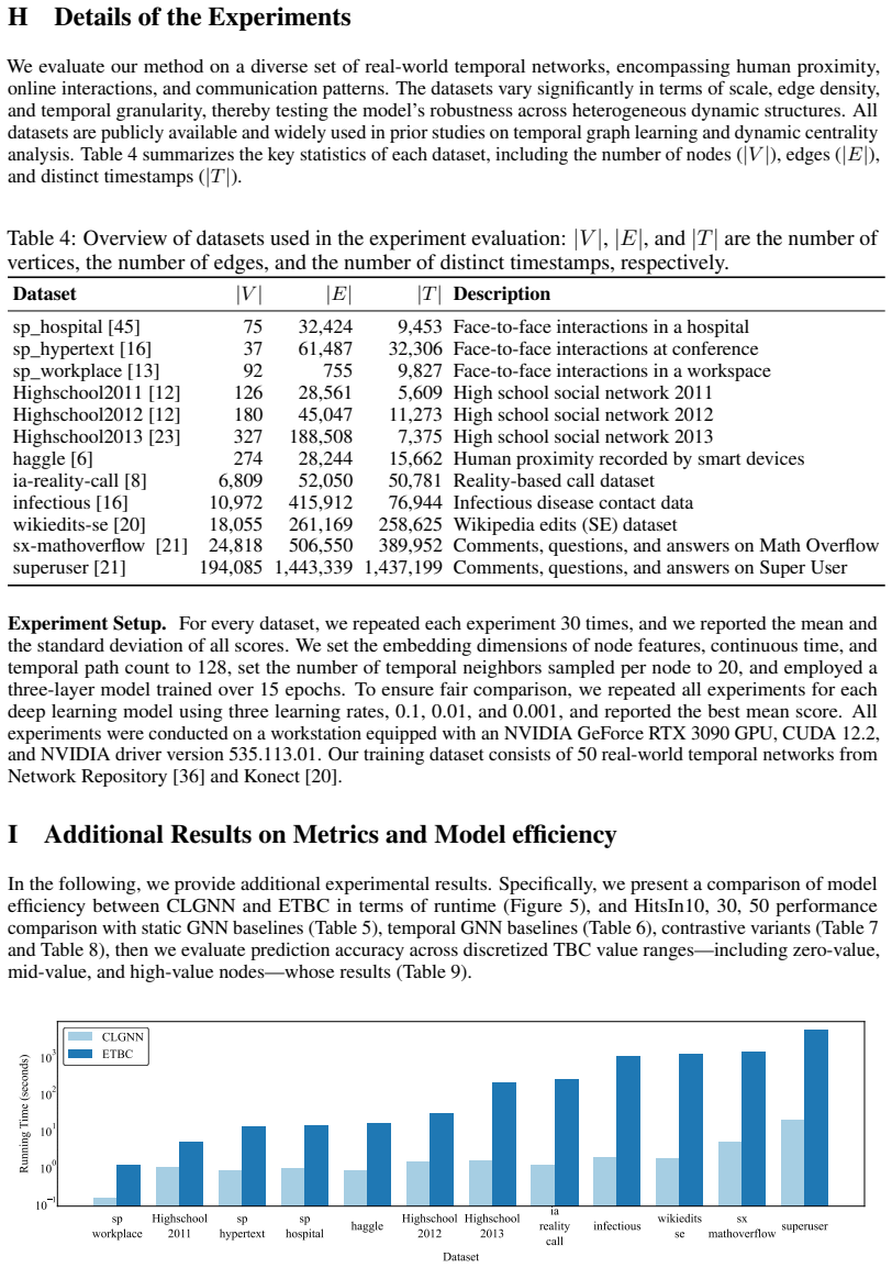
- Temporal betweenness centrality can be approximated on graphs large enough that exact computation is infeasible, with reported speedups of 4.8x to 663.7x over the exact ETBC algorithm.
- Important hubs in temporal networks can be identified rather than collapsed into the zero-centrality majority, because the contrastive module explicitly separates mid- and high-value nodes and improves Spearman ranking quality.
- The model works under multiple optimal path definitions, including shortest, shortest-plus-earliest-arrival, and shortest-plus-latest-departure-plus-earliest-arrival, so one network can serve different temporal semantics.
- Because the model is inductive, a model trained on small temporal graphs can be applied to unseen graphs, avoiding the per-graph retraining that transductive baselines such as DBGNN require.
- Contrastive learning, rather than oversampling, undersampling, Tweedie loss, or random graph augmentation, handles the extreme imbalance of centrality distributions on graphs.
Reading between the lines
- Beyond the paper, the same recipe — stability-selected clusters plus TBC-weighted contrastive pairs — should transfer to other imbalanced graph regression targets such as temporal closeness or Katz centrality, because the mechanism only assumes a skewed scalar label per node and an embedding space.
- The path-count gate $P(u,v,t)$ is a cheap proxy for temporal reachability; extending it to multi-step reachability counts could sharpen the signal on graphs with long time-respecting paths, a testable variation.
- If the 50 training networks and the exact train/test protocol are disclosed, the inductive claim can be directly verified by held-out evaluation; until then the cross-graph generalization claim is conditional on that protocol.
- The ablation results suggest that random graph augmentation hurts TBC prediction because it breaks time-respecting paths; a principled next step would be augmentation that edits only causally irrelevant edges.
Editorial analysis
A structured set of objections, weighed in public.
Referee Report
Summary. The paper proposes CLGNN, a contrastive-learning GNN for predicting temporal betweenness centrality (TBC). The model constructs an instance graph, augments node representations with temporal path counts and time encodings, uses a dual mean/attention aggregator, and couples a clustering-guided contrastive module (KContrastNet) with a regression head (ValueNet). The authors claim large accuracy gains over static and temporal GNN baselines and large speedups over exact TBC computation, based on 12 real datasets and 30 runs per experiment. The manuscript also includes ablation studies, hyperparameter analyses, and several theoretical appendices.
Significance. If the empirical claims are sound, the paper makes a useful contribution: it is an inductive, scalable TBC regressor rather than a transductive one, and the contrastive imbalance-handling design is a plausible remedy for the extreme skew in TBC distributions. The presentation of 30-run means with standard deviations, comparisons against the exact ETBC method, the fairness intuitions in Appendix F, and the multiple optimal-path-definition study are positive features. However, the headline numbers currently rest on an underspecified evaluation protocol: the 50 training graphs are unnamed, the train/test split is undefined, and learning-rate selection is reported as selecting the 'best mean score' without stating that a validation set was used. These issues must be resolved before the claimed improvements can be accepted.
major comments (4)
- [Section 5 (Datasets) and Appendix H] The paper claims that CLGNN is 'trained on small graphs and generalizes to unseen graphs', but the 50 real-world training networks are never named and no train/test split is described. To support the inductive-generalization claim, the authors must list the 50 training networks, explicitly state whether any of the 12 evaluation datasets in Table 4 overlap with them, and describe how the trained model is applied to each test graph.
- [Appendix H (Experiment Setup)] The paper states that for each deep learning model it tried three learning rates and 'reported the best mean score', but it does not state that this selection was performed on a validation split. If the best mean is selected by evaluating on the test set, the improvements in Tables 1 and 2 are systematically optimistic. The conclusion only says the learning rate was tuned via grid search. The authors must specify the selection protocol and, if selection was not validation-based, rerun the experiments with a proper validation split.
- [Section 5 and Appendix H] The experimental protocol does not describe how the 50-graph training corpus is used: is one model trained on all 50 graphs and then evaluated on each test graph, or is a separate model trained per test dataset with possible fine-tuning? It is also unclear how the transductive DBGNN baseline is adapted to the cross-graph setting. Without this information, the reported head-to-head gains cannot be attributed to inductive generalization rather than to different training setups.
- [Section 3 (Definition 2) and Section 5] TBC depends on the temporal-path parameter delta and on the chosen optimal-path definition, but the main experiments (Tables 1 and 2) do not state which definition and which delta value were used to compute ground-truth TBC. Appendix K shows that performance is highly sensitive to the path definition (e.g., sp_hypertext MAE ranges from 6.09 to 50.15), so the main tables are not reproducible without this information.
minor comments (6)
- [Abstract and Section 5 (RQ1)] The abstract reports up to 16.7x higher Spearman correlation, while the RQ1 discussion says 16.5x; these numbers should be harmonized.
- [Figure 1] The caption contains 'theia-reality-call'; this should be 'ia-reality-call'.
- [Conclusion] The text says 'real-world datesets'; this should be 'datasets'.
- [Appendix G] Proposition G.1 refers to 'Eq. (xx) of the main paper'; this placeholder should be resolved.
- [Appendix K] The phrase 'n contrast' should be 'In contrast'.
- [Section 4.1] The temporal path count P(u,v,t) is defined only via the number of later outgoing edges from v, not via actual path enumeration; the paper should explicitly acknowledge this is a heuristic proxy and discuss its limitations.
Circularity Check
No circularity: CLGNN is a supervised regressor whose TBC labels enter only through training losses and contrastive pair selection; the reported evaluation-protocol caveats are reliability concerns, not constructional circularity.
full rationale
CLGNN is a supervised regressor: ground-truth TBC values are used only in the training objective, through the regression loss L_regress and through the TBC-difference-based positive/negative pair construction and reweighting in KContrastNet; at inference ValueNet maps learned embeddings to TBC. No equation in Section 4 defines the prediction as a function of the labels or as a fitted constant, and the temporal path-count feature P(u,v,t) is a local reachability signal, not the normalized all-pairs TBC target, so the input is not the output under another name. The comparison baselines (GCN, DrBC, GNN-Bet, TGAT, TATKC, DBGNN, IIOIwD) are external systems, and the self-citations to TATKC [52], ETBC [53], and IIOIwD [54] serve as baseline methods, exact-computation ground truth, or speedup comparators rather than as uniqueness theorems or unverified premises that force the central claim. The main caveats—an unnamed 50-network training set with no disclosed split versus the 12 evaluation datasets, and the statement 'we repeated all experiments for each deep learning model using three learning rates, 0.1, 0.01, and 0.001, and reported the best mean score' (Appendix H) without an explicit validation split—are evaluation-reliability threats that could inflate the headline gains, but they do not make any prediction equivalent to its inputs by construction. Hence no significant circularity.
Assumptions & free parameters
free parameters (5)
- alpha (loss trade-off) =
0.2 (default)
- lambda (aggregation weight) =
0.4 (default)
- gamma_pos (positive threshold) =
0.5
- gamma_neg (negative threshold) =
0.5
- tau (temperature) =
not specified
assumptions (3)
- domain assumption The 12 evaluation datasets are representative of real-world temporal graphs and the exact TBC labels computed by ETBC are correct.
- standard math The bootstrap stability clustering estimate is consistent and the i.i.d. resampling assumption holds.
- ad hoc to paper The temporal path count P(u,v,t), defined as the number of outgoing edges from v with a later timestamp, is a sufficient proxy for path validity.
Cite this review
Pith. "Pith review of CLGNN: A Contrastive Learning-based GNN Model for Betweenness Centrality Prediction on Temporal Graphs." pith.science (2026). https://pith.science/paper/DZOY24FW
@misc{pith2026250614122,
  author       = {Pith},
  title        = {Pith review of: CLGNN: A Contrastive Learning-based GNN Model for Betweenness Centrality Prediction on Temporal Graphs},
  year         = {2026},
  howpublished = {\url{https://pith.science/paper/DZOY24FW}},
  note         = {Machine review of arXiv:2506.14122}
}
abstract
Temporal Betweenness Centrality (TBC) measures how often a node appears on optimal temporal paths, reflecting its importance in temporal networks. However, exact computation is highly expensive, and real-world TBC distributions are extremely imbalanced. The severe imbalance leads learning-based models to overfit to zero-centrality nodes, resulting in inaccurate TBC predictions and failure to identify truly central nodes. Existing graph neural network (GNN) methods either fail to handle such imbalance or ignore temporal dependencies altogether. To address these issues, we propose a scalable and inductive contrastive learning-based GNN (CLGNN) for accurate and efficient TBC prediction. CLGNN builds an instance graph to preserve path validity and temporal order, then encodes structural and temporal features using dual aggregation, i.e., mean and edge-to-node multi-head attention mechanisms, enhanced by temporal path count and time encodings. A stability-based clustering-guided contrastive module (KContrastNet) is introduced to separate high-, median-, and low-centrality nodes in representation space, mitigating class imbalance, while a regression module (ValueNet) estimates TBC values. CLGNN also supports multiple optimal path definitions to accommodate diverse temporal semantics. Extensive experiments demonstrate the effectiveness and efficiency of CLGNN across diverse benchmarks. CLGNN achieves up to a 663.7~$\times$ speedup compared to state-of-the-art exact TBC computation methods. It outperforms leading static GNN baselines with up to 31.4~$\times$ lower MAE and 16.7~$\times$ higher Spearman correlation, and surpasses state-of-the-art temporal GNNs with up to 5.7~$\times$ lower MAE and 3.9~$\times$ higher Spearman correlation.
Figures


Figures from the paper (3 more)


Reference graph
Works this paper leans on
-
[1]
M. Borassi and E. Natale. KADABRA is an adaptive algorithm for betweenness via random approximation. ACM J. Exp. Algorithmics, 24(1):1.2:1–1.2:35, 2019
work page 2019
-
[2]
U. Brandes. A faster algorithm for betweenness centrality.Journal of mathematical sociology, 25(2):163– 177, 2001
work page 2001
-
[3]
U. Brandes and C. Pich. Centrality estimation in large networks.Int. J. Bifurc. Chaos, 17(7):2303–2318, 2007
work page 2007
- [4]
-
[5]
S. Buß, H. Molter, R. Niedermeier, and M. Rymar. Algorithmic aspects of temporal betweenness. InKDD, pages 2084–2092, 2020
work page 2020
-
[6]
A. Chaintreau, P. Hui, J. Crowcroft, C. Diot, R. Gass, and J. Scott. Impact of human mobility on opportunistic forwarding algorithms.IEEE Transactions on Mobile Computing, 6(6):606–620, 2007
work page 2007
-
[7]
C. Cousins, C. Wohlgemuth, and M. Riondato. Bavarian: Betweenness centrality approximation with variance-aware rademacher averages. InSIGKDD, pages 196–206, 2021
work page 2021
-
[8]
N. Eagle and A. Pentland. Reality mining: sensing complex social systems.Personal and Ubiquitous Computing, 10(4):255–268, 2006
work page 2006
Show all 58 references
-
[9]
Erdös, V
D. Erdös, V . Ishakian, A. Bestavros, and E. Terzi. A divide-and-conquer algorithm for betweenness centrality. InSIAM, pages 433–441, 2015
2015
-
[10]
C. Fan, L. Zeng, Y . Ding, M. Chen, Y . Sun, and Z. Liu. Learning to identify high betweenness centrality nodes from scratch: A novel graph neural network approach. InCIKM, pages 559–568, 2019
2019
-
[11]
Fang and J
Y . Fang and J. Wang. Selection of the number of clusters via the bootstrap method.Computational Statistics & Data Analysis, 56(3):468–477, 2012
2012
-
[12]
Fournet and A
J. Fournet and A. Barrat. Contact patterns among high school students.PLoS ONE, 9(9):e107878, 2014. Data collected in collaboration with SocioPatterns. Seehttp://www.sociopatterns.orgfor details
2014
-
[13]
Génois and A
M. Génois and A. Barrat. Can co-location be used as a proxy for face-to-face contacts?EPJ Data Science, 7(1):1–18, 2018
2018
-
[14]
J. A. Hartigan and M. A. Wong. Algorithm as 136: A k-means clustering algorithm.Journal of the royal statistical society. series c (applied statistics), 28(1):100–108, 1979
1979
-
[15]
Heeg and I
F. Heeg and I. Scholtes. Using time-aware graph neural networks to predict temporal centralities in dynamic graphs. InNeurIPS, 2024
2024
-
[16]
Isella, J
L. Isella, J. Stehlé, A. Barrat, C. Cattuto, J. Pinton, and W. Van den Broeck. What’s in a crowd? analysis of face-to-face behavioral networks.Journal of Theoretical Biology, 271(1):166–180, 2011
2011
-
[17]
Jacob, D
R. Jacob, D. Koschützki, K. A. Lehmann, L. Peeters, and D. Tenfelde-Podehl. Algorithms for centrality indices. InNetwork Analysis, pages 62–82, 2004
2004
-
[18]
T. N. Kipf and M. Welling. Semi-supervised classification with graph convolutional networks, 2017
2017
-
[19]
Kourtellis, T
N. Kourtellis, T. Alahakoon, R. Simha, A. Iamnitchi, and R. Tripathi. Identifying high betweenness centrality nodes in large social networks.CoRR, abs/1702.06087, 2017
2017 arXiv
-
[20]
J. Kunegis. Konect: the koblenz network collection. InProceedings of the 22nd International Conference on World Wide Web, pages 1343–1350. ACM, 2013
2013
-
[21]
Leskovec and A
J. Leskovec and A. Krevl. Snap datasets: Stanford large network dataset collection. http://snap. stanford.edu/data, 2014. Accessed: 2025-05-12. 10
2014
-
[22]
Y . Li, Y . Xu, X. Lin, W. Zhang, and Y . Zhang. Ranking on dynamic graphs: An effective and robust band-pass disentangled approach. InProceedings of the ACM on Web Conference 2025, WWW ’25, page 3918–3929, New York, NY , USA, 2025. Association for Computing Machinery
2025
-
[23]
Mastrandrea, J
R. Mastrandrea, J. Fournet, and A. Barrat. Contact patterns in a high school: a comparison between data collected using wearable sensors, contact diaries and friendship surveys.PLoS ONE, 10(9):e0136497,
-
[24]
S. K. Maurya, X. Liu, and T. Murata. Fast approximations of betweenness centrality with graph neural networks. InCIKM, pages 2149–2152, 2019
2019
-
[25]
S. K. Maurya, X. Liu, and T. Murata. Graph neural networks for fast node ranking approximation.ACM Trans. Knowl. Discov. Data, 15(5):78:1–78:32, 2021
2021
-
[26]
M. R. F. Mendonça, A. Barreto, and A. Ziviani. Approximating network centrality measures using node embedding and machine learning.IEEE Trans. Netw. Sci. Eng., 8(1):220–230, 2021
2021
-
[27]
Pareja, G
A. Pareja, G. Domeniconi, J. Chen, T. Ma, T. Suzumura, H. Kanezashi, T. Kaler, T. Schardl, and C. Leiser- son. Evolvegcn: Evolving graph convolutional networks for dynamic graphs. InProceedings of the AAAI conference on artificial intelligence, volume 34, pages 5363–5370, 2020
2020
-
[28]
T. P. Peixoto. Netzschleuder: Network catalogue. https://networks.skewed.de/. Accessed: 2025- 05-12
2025
-
[29]
Pellegrina and F
L. Pellegrina and F. Vandin. SILV AN: estimating betweenness centralities with progressive sampling and non-uniform rademacher bounds.CoRR, abs/2106.03462, 2021
2021 arXiv
-
[30]
Pfeffer and K
J. Pfeffer and K. M. Carley. k-centralities: local approximations of global measures based on shortest paths. InWWW, pages 1043–1050, 2012
2012
-
[31]
Qarkaxhija, V
L. Qarkaxhija, V . Perri, and I. Scholtes. De bruijn goes neural: Causality-aware graph neural networks for time series data on dynamic graphs. InLearning on Graphs Conference, pages 51–1. PMLR, 2022
2022
-
[32]
S. C. Regunta, S. H. Tondomker, K. Shukla, and K. Kothapalli. Efficient parallel algorithms for dynamic closeness- and betweenness centrality.Concurr. Comput. Pract. Exp., 35(17), 2023
2023
-
[33]
Riondato and E
M. Riondato and E. M. Kornaropoulos. Fast approximation of betweenness centrality through sampling. Data Min. Knowl. Discov., 30(2):438–475, 2016
2016
-
[34]
Riondato and E
M. Riondato and E. Upfal. ABRA: approximating betweenness centrality in static and dynamic graphs with rademacher averages. InSIGKDD, pages 1145–1154, 2016
2016
-
[35]
Rossi, B
E. Rossi, B. Chamberlain, F. Frasca, D. Eynard, F. Monti, and M. M. Bronstein. Temporal graph networks for deep learning on dynamic graphs.CoRR, abs/2006.10637, 2020
2006 arXiv
-
[36]
R. A. Rossi and N. K. Ahmed. The network data repository with interactive graph analytics and visualiza- tion, 2015. Accessed: May 2025
2015
-
[37]
P. J. Rousseeuw. Silhouettes: a graphical aid to the interpretation and validation of cluster analysis.Journal of computational and applied mathematics, 20:53–65, 1987
1987
-
[38]
Sankar, Y
A. Sankar, Y . Wu, L. Gou, W. Zhang, and H. Yang. Dysat: Deep neural representation learning on dynamic graphs via self-attention networks. InWSDM, pages 519–527, 2020
2020
-
[39]
Santoro and I
D. Santoro and I. Sarpe. ONBRA: rigorous estimation of the temporal betweenness centrality in temporal networks. InWWW, pages 1579–1588, 2022
2022
-
[40]
A. E. Sariyüce, K. Kaya, E. Saule, and Ü. V . Çatalyürek. Graph manipulations for fast centrality computa- tion.ACM Trans. Knowl. Discov. Data, 11(3):26:1–26:25, 2017
2017
-
[41]
Saunshi, O
N. Saunshi, O. Plevrakis, S. Arora, M. Khodak, and H. Khandeparkar. A theoretical analysis of contrastive unsupervised representation learning. InInternational Conference on Machine Learning, pages 5628–5637. PMLR, 2019
2019
-
[42]
R. L. Thorndike. Who belongs in the family?Psychometrika, 18(4):267–276, 1953
1953
-
[43]
Tsalouchidou, R
I. Tsalouchidou, R. Baeza-Yates, F. Bonchi, K. Liao, and T. Sellis. Temporal betweenness centrality in dynamic graphs.Int. J. Data Sci. Anal., 9(3):257–272, 2020
2020
-
[44]
van den Oord, Y
A. van den Oord, Y . Li, and O. Vinyals. Representation learning with contrastive predictive coding.CoRR, abs/1807.03748, 2018
2018 arXiv
-
[45]
Vanhems, A
P. Vanhems, A. Barrat, C. Cattuto, J.-F. Pinton, N. Khanafer, C. Régis, B.-A. Kim, B. Comte, and N. V oirin. Estimating potential infection transmission routes in hospital wards using wearable proximity sensors. PloS one, 8(9):e73970, 2013
2013
-
[46]
S. Wang, W. Lin, Y . Yang, X. Xiao, and S. Zhou. Efficient route planning on public transportation networks: A labelling approach. InSIGMOD, pages 967–982, 2015. 11
2015
-
[47]
Wang and P
T. Wang and P. Isola. Understanding contrastive representation learning through alignment and uniformity on the hypersphere. InInternational conference on machine learning, pages 9929–9939. PMLR, 2020
2020
-
[48]
X. Wang, Y . Wang, X. Lin, J. X. Yu, H. Gao, X. Cheng, and D. Yu. Efficient betweenness centrality computation over large heterogeneous information networks.Proc. VLDB Endow., 17(11):3360–3372, 2024
2024
-
[49]
D. Xu, C. Ruan, E. Körpeoglu, S. Kumar, and K. Achan. Inductive representation learning on temporal graphs. InICLR, 2020
2020
-
[50]
Y . Yang, K. Zha, Y . Chen, H. Wang, and D. Katabi. Delving into deep imbalanced regression. InICML, 2021
2021
-
[51]
Zhang, R
Q. Zhang, R. Li, M. Pan, Y . Dai, G. Wang, and Y . Yuan. Efficient top-k ego-betweenness search. InICDE, pages 380–392, 2022
2022
-
[52]
Zhang, J
T. Zhang, J. Fang, Z. Yang, B. Cao, and J. Fan. TATKC: A temporal graph neural network for fast approximate temporal katz centrality ranking. InWWW, pages 527–538, 2024
2024
-
[53]
Zhang, Y
T. Zhang, Y . Gao, J. Zhao, L. Chen, L. Jin, Z. Yang, B. Cao, and J. Fan. Efficient exact and approximate betweenness centrality computation for temporal graphs. InWWW, pages 2395–2406, 2024
2024
-
[54]
Zhang, C
T. Zhang, C. Hou, R. Jiang, X. Zhang, C. Zhou, K. Tang, and H. Lv. Label informed contrastive pretraining for node importance estimation on knowledge graphs.IEEE Transactions on Neural Networks and Learning Systems, 36(3):4462–4476, 2025
2025
-
[55]
…𝒗𝟐 𝒗𝟑 𝒗𝟒 𝑡&𝑡'𝑡( 𝑡)𝑡* 𝑡*𝑡+ [𝑡
Y . Zou, T. Li, and Z. Luo. Node centrality approximation for large networks based on inductive graph neural networks.CoRR, abs/2403.04977, 2024. 12 A Details of the CLGNN——Representation Module As shown in Figure 3, the representation module integrates structural and temporal...
2024 arXiv
-
[57]
The positive-pair weightβ uv is strictly decreasing with respect to∆ uv
-
[58]
Proof.• Forβ uv = T BCmedian ·γ pos ∆uv , we have: dβuv d∆uv =− T BCmedian ·γ pos ∆2uv <0
The negative-pair weightβ uw is strictly increasing with respect to∆ uw. Proof.• Forβ uv = T BCmedian ·γ pos ∆uv , we have: dβuv d∆uv =− T BCmedian ·γ pos ∆2uv <0. Hence, βuv decreases as the TBC difference increases, emphasizing the similarity of closely matched pairs. • Forβ...
2011
-
[2015]
See http://www.sociopatterns.org for details
Data collected in collaboration with SocioPatterns. See http://www.sociopatterns.org for details
Reviewed August 7, 2026 · model on record in the stance chip above.
Discussion (0). Sign in to comment.