Geometric sensitivity of modal parameters in wind instrument models: a case study on saxophone intonation

Christophe Vergez (LMA); Micha\"el Jousserand; Nathan Szwarcberg (LMA); Tom Colinot

Geometric sensitivity of modal parameters in wind instrument models: a case study on saxophone intonation

T0 review · 0 major / 7 minor · reviewed 2026-08-06 · deepseek-v4-flash

Challenge this review Re-run · record.json Download PDF Read on arXiv ↗ Review JSON

Pith's one-line read For a transfer-matrix resonator, every pole's derivative with respect to a geometric parameter is a closed-form ratio of partial derivatives of the impedance denominator, so modal parameters can be updated analytically without re-solving…

desk verdict Solid, honest paper: the math is standard but the residue sensitivities and TMM framework are new, the validation is careful, and the simplified saxophone limits the tuning advice but not the method. read the letter →

arxiv 2506.16220 v3 pith:PEHENA44 submitted 2025-06-19 physics.class-ph

Nathan Szwarcberg (LMA) , Tom Colinot , Christophe Vergez (LMA) , Michaël Jousserand This is my paper · ORCID

classification physics.class-ph

keywords TransferMatrixMethodmodalparametersanalyticsensitivityimplicitdifferentiationwindinstrumentacousticssaxophoneintonationregisterholeinharmonicity

verification ladder T0 review T1 audit T2 compute T3 formal

The pith

A machine-rendered reading of the paper's core claim, the machinery that carries it, and where it could break.

The reading

The paper establishes that when a wind-instrument resonator is modeled by the Transfer Matrix Method, the modal parameters—complex resonance frequencies (poles) and their amplitudes (residues)—are implicitly defined functions of every geometric dimension, and their derivatives with respect to those dimensions can be written as closed-form ratios of partial derivatives of the impedance denominator. Concretely, a pole $s_n$ satisfying $D(s_n,\theta)=0$ obeys $ds_n/d\theta = -(\partial D/\partial\theta)/(\partial D/\partial s)$, and an analogous formula holds for the residue $C_n$. This turns the transfer-matrix model into a source of analytic gradients, so small changes in bore length, hole radius, or chimney height can be converted directly into predicted shifts in cents, without re-solving the resonance equation. The authors apply the machinery to a simplified soprano saxophone, producing per-note sensitivity curves for the register hole and testing a first-order optimization that reduces the worst second-register inharmonicity. If the claims hold, instrument makers can use these gradients as quantitative guidance for tuning adjustments, and time-domain sound synthesis can update modes smoothly as geometry changes over time.

What carries the argument

The load-bearing object is the implicit-function-theorem derivative of the impedance denominator $D(s,\theta)$, assembled from the product of elementary transfer matrices for cylinders, cones, toneholes, and radiation. The pole sensitivity formula $ds_n/d\theta = -(\partial D/\partial\theta)/(\partial D/\partial s)$ carries the argument; everything else in the paper is an application or verification of this identity in the form of residue derivatives, inharmonicity gradients in cents per millimeter, and first-order predictions of pole motion. Automated symbolic differentiation with generated numerical evaluation code is the practical enabler that makes the gradients usable in parameter sweeps and optimization loops.

What would settle it

Run the minimal working example and repeat the paper's downstream-hole test: reduce the register-hole radius by 0.2 mm, solve $D(s_n,\theta+\Delta\theta)=0$ exactly for the new poles, and compare the resulting inharmonicity with the sensitivity-based prediction of a 3.4-cent improvement at D4/D5; a mismatch far beyond first-order error would falsify the sensitivity chain. A second check is to take a geometry with two nearly coincident poles, where $D'(s_n)\approx0$; the formula predicts a very large or divergent sensitivity, and exact pole computation should show the two modes merging.

Watch

Extended reading notes

Core claim

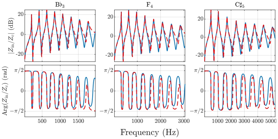
The central discovery is a differentiation identity for modal parameters of transfer-matrix resonators. Since the input impedance is a ratio $Z_{in}=N(s)/D(s)$ of analytic functions and the poles are roots of $D(s_n,\theta)=0$, the implicit function theorem gives $ds_n/d\theta = -(\partial D/\partial\theta)/(\partial D/\partial s)$ at the pole, and differentiating $C_n=N(s_n,\theta)/D'(s_n,\theta)$ yields the residue sensitivity, including the pole's own movement term. The paper verifies these sensitivities by stepping the cone length from 190 mm to 750 mm and comparing first-order updates against exact pole computations, finding relative errors below 0.6% for the poles; it then computes the derivative of register inharmonicity $h(s_1^{(c)},s_2^{(o)})=1200\log_2\!\left(\frac{\Im(s_2^{(o)})}{2\,\Im(s_1^{(c)})}\right)$ with respect to each geometric parameter and uses those sensitivity curves to reduce inharmonicity in a test optimization.

Load-bearing premise

The tuning recommendations for a real soprano saxophone assume the simplified resonator—a truncated cone with a single register hole, a cylindrical mouthpiece, and linear losses—behaves enough like the physical instrument; the derivative formulas themselves do not depend on that assumption.

Editorial extensions

If this is right

Any resonator expressible as a transfer-matrix product gains a closed-form gradient for every pole and residue, so modal parameters can be updated without re-solving the resonance equation.
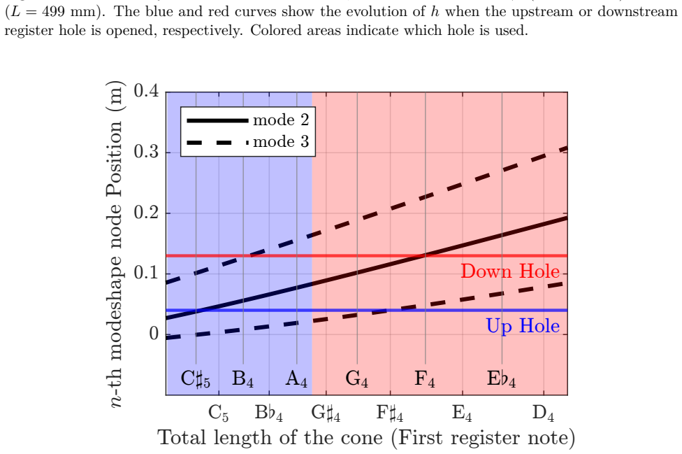
Sensitivity curves for register inharmonicity give instrument makers a per-note, per-millimeter map of which geometric changes improve intonation and which worsen it, with the zero-crossings tied to pressure-node positions.
For time-varying geometry in sound synthesis—a trombone slide, a glissotar, or opening side holes—modes can be updated at each time step using the analytic derivatives.
First-order sensitivity stays accurate for large pole excursions (below 0.6% relative error after the cone length grows from 190 mm to 750 mm), but large parameter changes such as doubling a chimney height require higher-order or predictor-corrector corrections.
The same sensitivity functions extend naturally to other modal quantities, including damping ratio or the frequency ratio of the first two impedance peaks that governs whether a register hole overblows.

Reading between the lines

Editorial extensions of the paper, not claims the author makes directly.

Beyond the paper's note-by-note treatment, the same analytic gradients could drive a multi-objective optimizer that tunes all twelve note pairs at once, trading register-hole parameters against global bore shape.
The implicit-differentiation identity is not specific to acoustics: any transfer-matrix model with a rational impedance—electromagnetic or structural waveguides, for example—would carry the same modal sensitivity formula.
A testable extension the paper only touches on: the threshold where a register hole stops overblowing (around $R_h\le0.5$ mm on a cylindrical tube) should appear as a sign change or divergence in the sensitivity of the frequency ratio $\Im(s_2^{(o)})/\Im(s_1^{(o)})$, which an experiment could confirm.
Because the pole and residue gradients are available, stability of oscillating regimes under geometry changes could be assessed by coupling these sensitivities to a nonlinear continuation model, telling makers not only how many cents a change saves but whether the second register still speaks.

Share X Bluesky LinkedIn Reddit HN

Editorial analysis

A structured set of objections, weighed in public.

Desk editor's note, referee report, and a circularity audit.

Desk Editor's Note

read the letter

This is a clean, honest paper. The pole sensitivity formula is textbook implicit differentiation, but the residue sensitivity and the systematic TMM treatment with viscothermal losses and radiation are a real extension, and the symbolic-computation wrapper makes it usable. The derivation is correct and clearly presented. The validation via first-order continuation over 560 steps is appropriate, and the pole errors below 0.6% are reassuring. The optimization example is genuinely honest: the downstream Rh prediction works, the upstream Lh prediction fails as expected for a 100% parameter change, and they say so. The mode-shape analysis connecting register-hole position to pressure nodes gives intuitive grounding. They also ship a minimal working example on Zenodo, which is real value.

Soft spots: the demonstrated case is a simplified saxophone (truncated cone, one register hole, no tonehole lattice), so the tuning recommendations don't transfer directly to a physical instrument. The authors are upfront about this, and it doesn't threaten the central method. The modal decomposition itself shows larger errors at higher modes (up to 11% amplitude at the eighth peak), a known limitation of modal truncation, but worth noting. Also, residue sensitivities are less accurate than pole sensitivities; they acknowledge this and show that recomputing residues from the estimated poles helps. That is a minor caveat, not a flaw.

The citation pattern looks honest: they cite prior sensitivity work (Nederveen, Facchinetti, Ernoult) and correctly attribute the pole formula to implicit differentiation. The residue sensitivity and TMM-specific formulation are theirs, and self-citations are for prior model verification, not to inflate novelty.

Bottom line: this is a useful tool paper for musical acoustics and TMM users. It deserves a serious referee; the main points to probe are the accuracy limits of residue sensitivities and the practical validity of the simplified saxophone. I'd bring it to a reading group and would cite it if I worked in this area.

Referee Report

0 major / 7 minor

Summary. The paper derives analytic sensitivities of the modal parameters (complex poles and residues) of a one-dimensional waveguide modeled by the Transfer Matrix Method with respect to geometric parameters. The central formulas, Eqs. (7) and (8), follow from implicit differentiation of the denominator and residue definitions. The method is validated by comparing first-order Euler updates of poles and residues against direct numerical solution of the TMM characteristic equation over 560 steps, with reported errors below 0.6% for poles. The application is a simplified model of a soprano saxophone, where the sensitivity of octave inharmonicity to register-hole position, radius, chimney height, input radius, and cone angle is computed and used in a small optimization example. The paper also demonstrates the use of symbolic differentiation to generate efficient sensitivity functions and provides a minimal working example on Zenodo.

Significance. If accepted, the paper provides a clean and general analytical tool: for any TMM resonator, the derivative of a pole or residue with respect to a parameter is obtained without re-solving the characteristic equation. This is useful for instrument design, optimization, and time-domain synthesis with time-varying geometry. Strengths include the correct and transparent derivation, the numerical consistency check against direct TMM solutions, the honest reporting of where first-order predictions fail (e.g., the upstream-hole chimney-length example in Section 3.3), and the availability of a reproducible minimal implementation. The main limitation, that the saxophone case study uses a simplified geometry with a single register hole and no tonehole lattice, is explicitly stated in the abstract, Section 3, and Figure 1; it limits transfer of the specific tuning recommendations to a physical instrument but does not affect the correctness of the sensitivity formalism. The paper's claims are appropriately scoped, and the acknowledged simplifications and failure modes are weighed fairly in the discussion.

minor comments (7)

[§3.3] In the sentence describing the upstream-hole chimney-length test, the text appears corrupted as 'A4mmincreaseistested'; it should read 'A 4 mm increase is tested.'
[§2.1] Just before Eq. (4), the phrase 'thepreviousexpression' lacks spaces and should be corrected to 'the previous expression'.
[Appendix] The reference 'Lefevbre' is a typo for 'Lefebvre'; also, the symbol R⊙ is used in the radiation-model sentence without being defined in the list of symbols.
[Figure 3] The axis labels contain rendering artifacts such as 'Conelength' and '=(sn)/(2:)' that should be corrected in the production version.
[§2.2 and §4] The claim that the analytical derivatives can be extended to arbitrary order is stated but not substantiated with a formula or example; adding the second-order expression or a brief explanation would support this assertion.
[§3.1] The validation compares the sensitivity-based predictions against direct computations of the same TMM model; adding one sentence that this is a numerical consistency check rather than an experimental benchmark would help readers interpret the scope.
[Table 1] The column header 'Effectivity (Notes)' is unusual; 'Effective range (notes)' or 'Applies to notes' would be clearer.

Circularity Check

0 steps flagged · score 0.0 of 10

No significant circularity: the sensitivity derivation is self-contained and the self-citations are not load-bearing.

full rationale

The central claim (Eqs. 7 and 8) is obtained by implicit differentiation of the defining equation D(s_n(θ), θ) = 0 and the residue formula C_n = N/D'. This is a self-contained mathematical derivation, not an input recycled as a prediction. The validations in Sec. 3.1 and Fig. 8 compare first-order sensitivity predictions against direct numerical solution of Eq. (2) for the same TMM model; that is a benchmark against the model's own exact solve, which is legitimate verification of the derivative formula and involves no fitted parameters. The measured saxophone parameters in Table 1 are model inputs, not tuned to match the inharmonicity predictions. Self-citations (e.g., mode-shape details in [szwarcberg2024second], the Rh overblow observation, and Appendix model references) are supporting or peripheral and do not supply the central sensitivity result. The simplified cone-plus-one-hole geometry limits practical transferability of tuning advice, but the paper explicitly labels the model as simplified and correctly scopes the claim; this is a modeling limitation, not circularity.

Assumptions & free parameters 0 free parameters · 6 assumptions · 0 invented entities

The method itself rests on standard calculus (implicit function theorem) and on literature transfer matrix models. The case study's practical conclusions rest on the simplified saxophone geometry, which is a modeling assumption rather than a validated representation of a real instrument. No free parameters were fitted to the target; all geometry values in Table 1 come from measurements on a real soprano saxophone. No new entities are introduced.

assumptions (6)

standard math Implicit function theorem and differentiability of D(s,θ) with respect to s and θ, with simple poles (∂D/∂s ≠ 0).
Assumed in Section 2.2, Eqs. (6)-(7); required for the sensitivity formulas. The paper notes D differentiable and ∂D/∂s ≠ 0.
domain assumption One-dimensional plane wave propagation and viscothermal loss modeling via complex wavenumber Γ.
Standard TMM assumption, stated in Section 2.1; supports the transfer matrix models.
domain assumption The cited transfer matrix models for cylinders, cones, and toneholes, and the radiation impedance models, are accurate.
Relied on in the Appendix for all numerical results.
domain assumption The simplified saxophone geometry (truncated cone, one register hole, cylindrical mouthpiece) adequately represents a real soprano saxophone for second-register intonation.
Introduced in Section 3 and Figure 1; load-bearing for the case-study conclusions.
domain assumption The cylindrical mouthpiece length is set to Lcyl = R1/(3 tan φ) to match the volume of the missing cone tip.
A paper-specific modeling simplification, stated in Eq. (9), that does not force the target result.
domain assumption The register hole and open end radiation are modeled as infinitely flanged and unflanged, respectively.
Stated in the Appendix; an approximation that affects sensitivity values.

how reviews work

0 comments

Cite this review

Pith. "Pith review of Geometric sensitivity of modal parameters in wind instrument models: a case study on saxophone intonation." pith.science (2026). https://pith.science/paper/PEHENA44

@misc{pith2026250616220,
  author       = {Pith},
  title        = {Pith review of: Geometric sensitivity of modal parameters in wind instrument models: a case study on saxophone intonation},
  year         = {2026},
  howpublished = {\url{https://pith.science/paper/PEHENA44}},
  note         = {Machine review of arXiv:2506.16220}
}

read the original abstract

The Transfer Matrix Method is a practical approach for modeling plane wave propagation in one-dimensional waveguides. Its simplicity makes it especially attractive for accounting for viscothermal losses, enabling realistic simulations of complex waveguides such as wind instruments. Another strength of this method lies in its fully analytical formulation of wave propagation. Modal parameters naturally arise as by-products of the model, obtained by numerically solving analytical expressions. In this work, the analytical potential of the method is extended by deriving the sensitivity of modal parameters to changes in the geometry of the resonator. These analytical gradients are applied in the context of wind instrument design. A simplified model of a soprano saxophone is used to investigate how octave harmonicity can be optimized through small geometric adjustments. The proposed approach enables predictive adjustments of geometry and offers valuable insight for both sound synthesis and instrument making.

Figures

Figures reproduced from arXiv: 2506.16220 by the authors.

**Figure 1.** Scheme of the simplified saxophone. When the register hole is closed, the player produces notes near the first resonance frequency. This is the first register, noted R1 (c) (closed hole). When the register hole is open, notes close to the second resonance frequency are preferably produced. This is the second register, noted R (o) 2 (open hole). In an idealized conical resonator, the second register note is an octave… view at source ↗

**Figure 2.** Modulus and phase of the input impedance. Blue lines: direct computation from the TMM. [PITH_FULL_IMAGE:figures/full_fig_p008_2.png] view at source ↗

**Figure 3.** Variation of the modal coefficients sn and Cn, when the length of the cone L increases. Blue, red, yellow and purple curves refer to modes 1 to 4 respectively. Dashed lines show the explicit estimation of the modal coefficients through the sensitivity functions dsn/dL and dCn/dL. 3.2 Sensitivity curves for an intuitive optimization of second-register tuning [PITH_FULL_IMAGE:figures/full_fig_p009_3.png] view at source ↗

Figures from the paper (5 more)

**Figure 4.** Figure 4: Inharmonicity h between R2(o) and R1(c) , for all notes between C♯5 (L = 197 mm) and D4 (L = 499 mm). The blue and red curves show the evolution of h when the upstream or downstream register hole is opened, respectively. Colored areas indicate which hole is used. C5 B[…

**Figure 5.** Figure 5: Location of pressure nodes for the second (solid black line) and third mode (dashed black [PITH_FULL_IMAGE:figures/full_fig_p010_5.png]

**Figure 6.** Figure 6: Sensitivity of the inharmonicity h to small changes in L1, Rh, and Lh (in cents per mm). Rows correspond to the parameter varied. Left column: upstream hole. Right column: downstream hole. Thin black (y ≈ 0): sensitivity of first-register notes. Thin colored: second-re…

**Figure 7.** Figure 7: Sensitivity of inharmonicity h to small changes in R1 (first row) and φ (second row). Left: upstream hole. Right: downstream hole. Thin black: sensitivity of first-register notes. Thin colored: second-register notes. Thick colored: difference between second- and first-…

**Figure 8.** Figure 8: Incremental optimization of inharmonicity using sensitivity curves. For the upstream register [PITH_FULL_IMAGE:figures/full_fig_p014_8.png]

Discussion (0). Continue with ORCID to comment.

Reference graph

Works this paper leans on

4 extracted references · 4 canonical work pages

[1]

Geometric sensitivity of modal parameters in wind instrument models: a case study on saxophone intonation

Geometric sensitivity of modal parameters in wind instrument models: a case study on saxophone intonation Nathan Szwarcberga, b∗, Tom Colinota, Christophe Vergezb, Michaël Jousseranda a Buffet Crampon, 5 Rue Maurice Berteaux, 78711 Mantes-la-Ville, France b Aix Marseille Univ, CNRS, Centrale Med, LMA, Marseille, France Submitted to Acta Acustica, June 20,...

work page Pith review arXiv 1969
[2]

(2) can be solved analytically

(2) In the absence of losses and for simple geometries, Eq. (2) can be solved analytically. For more realistic models, it is solved numerically from appropriate initial conditions. Each complex polesn is related to a resonance frequencyfn, with: 2πfn =ℑ(sn). The residueCn at each pole is defined as the first-order coefficient in the Laurent expansion of Z...

work page 2010
[3]

Table 1: Initial parameters of the simplified soprano saxophone

They were measured on a real soprano saxophone. Table 1: Initial parameters of the simplified soprano saxophone. The temperature is fixed atT0 = 20◦C. The two cases correspond to the two register holes of the saxophone. φ (◦) R1 (mm) L1 (mm) Rh (mm) Lh (mm) Effectivity (Notes) Upstream hole 1.74 4.6 40 0.85 4.0 [A4; F♯5] Downstream hole 1.74 4.6 130 1.4 4...

work page 2024
[4]

• Theexpressionof Mcyl isgiveninChap.4.5ofChaigneandKergomard(2016)[ bible2016]

The complete model is made of a transfer matrixMtot, so that Mtot =McylMc1MhMc2. • Theexpressionof Mcyl isgiveninChap.4.5ofChaigneandKergomard(2016)[ bible2016]. • Theexpressionof Mhole canbefoundinLefevbreandScavone(2012)[ lefebvre2012characterization]. • The expression of the transfer matrix of a cone can be found in Tournemenne and Chabassier (2019) [t...

work page 2016

Pith tools

Reviewed August 6, 2026 · model on record in the stance chip above.

[1] [1]

Geometric sensitivity of modal parameters in wind instrument models: a case study on saxophone intonation

Geometric sensitivity of modal parameters in wind instrument models: a case study on saxophone intonation Nathan Szwarcberga, b∗, Tom Colinota, Christophe Vergezb, Michaël Jousseranda a Buffet Crampon, 5 Rue Maurice Berteaux, 78711 Mantes-la-Ville, France b Aix Marseille Univ, CNRS, Centrale Med, LMA, Marseille, France Submitted to Acta Acustica, June 20,...

work page Pith review arXiv 1969

[2] [2]

(2) can be solved analytically

(2) In the absence of losses and for simple geometries, Eq. (2) can be solved analytically. For more realistic models, it is solved numerically from appropriate initial conditions. Each complex polesn is related to a resonance frequencyfn, with: 2πfn =ℑ(sn). The residueCn at each pole is defined as the first-order coefficient in the Laurent expansion of Z...

work page 2010

[3] [3]

Table 1: Initial parameters of the simplified soprano saxophone

They were measured on a real soprano saxophone. Table 1: Initial parameters of the simplified soprano saxophone. The temperature is fixed atT0 = 20◦C. The two cases correspond to the two register holes of the saxophone. φ (◦) R1 (mm) L1 (mm) Rh (mm) Lh (mm) Effectivity (Notes) Upstream hole 1.74 4.6 40 0.85 4.0 [A4; F♯5] Downstream hole 1.74 4.6 130 1.4 4...

work page 2024

[4] [4]

• Theexpressionof Mcyl isgiveninChap.4.5ofChaigneandKergomard(2016)[ bible2016]

The complete model is made of a transfer matrixMtot, so that Mtot =McylMc1MhMc2. • Theexpressionof Mcyl isgiveninChap.4.5ofChaigneandKergomard(2016)[ bible2016]. • Theexpressionof Mhole canbefoundinLefevbreandScavone(2012)[ lefebvre2012characterization]. • The expression of the transfer matrix of a cone can be found in Tournemenne and Chabassier (2019) [t...

work page 2016