REVIEW 3 major objections 6 minor 48 references
ECLEIRS: Exact conservation law embedded identification of reduced states for parameterized partial differential equations from sparse and noisy data
T0 review · 3 major / 6 minor · reviewed 2026-08-15 · deepseek-v4-flash
Pith's one-line read Writing solution and flux as row-wise divergences of a skew-symmetric field makes reduced-state predictions conserve exactly, even for parameters absent from training.
desk verdict Useful combination of divergence-free potentials and INR reduced states, but the exact-conservation claim applies to the modeled flux pair, not the physical flux; worth a serious referee after honest reframing. read the letter →
The pith
A machine-rendered reading of the paper's core claim, the machinery that carries it, and where it could break.
The reading
What carries the argument
The load-bearing object is the space-time divergence-free ansatz: for a $d$-dimensional spatial domain one introduces a skew-symmetric matrix field $A(w;\mu)\in\mathbb{R}^{(d+1)\times(d+1)}$ and sets $z^m=(q^m,f^m)^T$ to the row-wise divergence of $A$. Because row-wise divergences of skew-symmetric matrices have zero space-time divergence, the conservation law is embedded in the model form itself. The entries $a(w;\mu)$ are decoded by an autodecoder MLP from reduced states $\tilde q(\mu,t)=h_\theta(\mu,t)$, and the reduced-state dynamics are identified by fitting a neural ODE to automatic-differentiation derivatives. This design is what transfers exact conservation to the inference stage, as any predicted $\tilde q$ still maps into the space of divergence-free lifted fields. The paper notes the modeled flux $f^m$ is learned as an independent field and need not equal the physical flux $f(q^m)$; the exactly enforced law is $\partial_t q^m+\nabla\cdot f^m=0$.
What would settle it
Evaluate the residual $\partial q^m/\partial t+\nabla\cdot f(q^m)$ with the true constitutive flux (for example, $c q^m$ for advection or $\tfrac{1}{2}c(q^m)^2$ for Burgers) at validation parameters outside the training set; if this residual is far above machine precision while the modeled-flux residual is at machine precision, the exact conservation claim holds only for the learned flux pair, not for the physical conservation law.
Extended reading notes
Core claim
The discovery is that exact conservation and data-driven dimensionality reduction can be combined without any tunable penalty: take the lifted space-time vector $z^m=(q^m,f^m)^T$ and define it as the row-wise divergence of a skew-symmetric matrix field $A(w;\mu)$. The divergence of a row-wise divergence of a skew-symmetric matrix is identically zero, so $\partial q^m/\partial t + \nabla\cdot f^m=0$ is satisfied to machine precision for any space-time point and any system parameter, whether or not that parameter appeared in training. The entries of $A$ are generated by an implicit neural representation conditioned on latent states $\tilde q(\mu,t)$ produced by a hypernetwork, and the latent dynamics are learned as a parameterized neural ODE. The same construction guarantees local subdomain and global conservation of the integrated modeled solution by the divergence theorem. On the three shock-propagation test problems, the authors find ECLEIRS gives the most accurate predictions for unseen parameters under sparse and noisy data, with conservation errors around $10^{-8}$ in single precision.
Load-bearing premise
The guarantee is built for the learned flux, which can differ from the true physical flux; if the learned flux drifts away from the real one, conservation of the modeled pair does not imply the physics is conserved.
Editorial extensions
If this is right
- Exact conservation becomes a hard guarantee of the reduced model, so forecasts for parameters or times outside the training window cannot drift out of the divergence-free constraint.
- No penalty parameter needs tuning; the physics constraint is not a soft loss term whose strength depends on noise level or problem.
- The mesh-free implicit representation lets the same reduced model ingest sparse sensor data and evaluate on any space-time locations, including different resolutions in offline and online stages.
- The divergence theorem turns the pointwise constraint into local subdomain and global conservation of integrated quantities, which is the property many applications actually need.
- The forecast stage inherits the guarantee because reduced states always map through the same divergence-free decoder after neural-ODE time integration.
Reading between the lines
- Editorial extension: the machine-precision conservation is established for the modeled pair $(q^m,f^m)$; whether the physical flux $f(q^m)$ satisfies the law is a separate, empirical question, and the paper's conservation metric in Eq. (30) uses the physical flux, so this is checkable.
- Editorial extension: because the potential formulation is linear, the method could be extended to coupled conservation systems by assigning each equation its own skew-symmetric potential, with a consistency penalty across shared variables as the paper suggests.
- Editorial extension: the exact constraint may act as an implicit regularizer that explains much of the denoising gain; a clean ablation training the same architecture with the consistency loss but without divergence-free structure would isolate this effect.
Signed reviews
Editorial analysis
A structured set of objections, weighed in public.
Referee Report
Summary. The manuscript introduces ECLEIRS, a reduced/latent state dynamics method for parameterized PDEs that represents the modeled solution q^m and flux f^m as the row-wise divergence of a skew-symmetric matrix field A(w;μ) whose components are decoded from latent states via an implicit neural representation (Section 3.2, Eqs. (13)-(20)). This construction implies the modeled pair satisfies ∂q^m/∂t + ∇·f^m = 0 identically. The method is evaluated on 1-D advection, 1-D Burgers, and 2-D Euler problems for two tasks: recovering clean signals from sparse/noisy data and predicting dynamics at parameters unseen during training, with comparisons against unconstrained (IRS) and penalty-based physics-informed (PI-IRS) baselines across several sparsity and noise levels.
Significance. The idea of embedding a divergence-free ansatz into an INR-based latent dynamics model is a useful and timely contribution; the space-time divergence-free parametrization is clearly explained, and the benchmark study is extensive, covering three shock-propagation problems with varying sparsity, noise, interpolation, and extrapolation settings. The practical advantage that ECLEIRS avoids the penalty-parameter tuning required by PI-IRS is well supported by the experiments. However, the headline theoretical claim that the governing physical conservation law is satisfied exactly for unseen parameters is not established: the construction guarantees conservation only for the modeled flux pair, because f^m is an independent field with f^m ≠ f(q^m), as the manuscript itself states in Section 3.2. Once this distinction is made explicit, the empirical observation that physical residuals are O(1e-8) for advection and Burgers remains valuable, but it is a numerical finding rather than a structural guarantee.
major comments (3)
- [Section 3.2, Eqs. (13)-(22); abstract; Section 5.1.2] The exact-conservation guarantee applies to the modeled pair (q^m, f^m), not to the physical law ∂q^m/∂t + ∇·f(q^m) = 0. The manuscript states in Section 3.2 that 'as the flux is also modeled as f^m, therefore f^m ≠ f(q^m)', so the space-time divergence-free construction does not by itself enforce the governing conservation law. The abstract's claim that ECLEIRS 'satisfies conservation laws exactly even for parameters unseen' and the similar statements in Sections 5.1.2 and 5.2.2 should be restricted to the modeled flux, and the machine-precision physical residuals reported in Figures 7 and 15 should be explicitly presented as empirical results rather than as consequences of the architecture.
- [Section 5.3, Eq. (35)] For the 2-D Euler problem, only the continuity equation ∂ρ/∂t + ∇·(ρu) = 0 is embedded in ECLEIRS and PI-IRS; momentum and energy conservation are not enforced. The manuscript should state this limitation wherever global statements such as 'satisfies conservation laws exactly' appear, and the conclusion should not imply that all conservation laws of the Euler system are satisfied.
- [Section 3.2 and Section 6] The inconsistency between the modeled flux and the physical flux is acknowledged in Section 3.2 and deferred to future work in Section 6, but it is central to interpreting the method's guarantees. Because the exactness property holds for a different flux, the paper should report the consistency error ||f^m - f(q^m)|| on the training and validation sets, or otherwise quantify how close the learned flux is to the physical flux. Without such a quantification, the small physical residuals in the advection and Burgers experiments are difficult to interpret and the theoretical contribution remains incomplete.
minor comments (6)
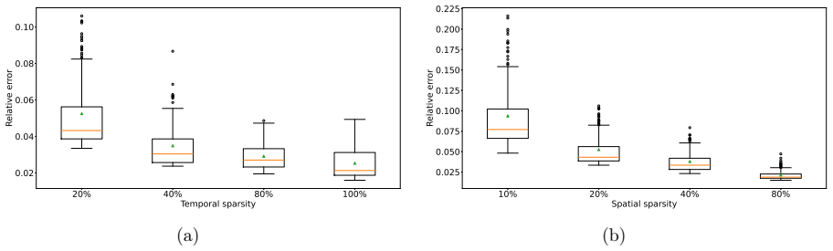
- [Figure 1 and Figure 19 captions] The captions refer to panel '(e)100% sparsity', but only panels (a)-(c) appear in both figures; please correct the panel references.
- [Table 4] The third parameter column is labeled 'xin', but the Burgers problem uses ω as the third parameter; please fix the header.
- [Section 5.2.1] The phrase 'an anamalous behavior' contains a typo; it should read 'an anomalous behavior'.
- [Figure 20 caption] The caption contains the typo 'groundn truth'; it should read 'ground truth'.
- [Equation (22)] The equation appears with garbled repeated arguments 'qqqm(t,x;µt,x;µt,x;µ)'; please fix the typesetting so that the argument is written consistently as (t,x;μ).
- [Section 5.1.1] The description of ECLEIRS as 'parameter-free' is only true with respect to the penalty parameter λ; the method still depends on architecture sizes and latent dimension. Please qualify the wording to avoid overclaiming.
Circularity Check
Exact conservation is a definitional property of the modeled flux pair, not of the physical flux; the abstract's 'governing conservation law' claim conflates the two.
-
self definitional
[Section 3.2 (Eqs. 13 and 16) and Section 3.4 (Eq. 22); abstract]
"Through algebraic manipulation, it is observed that these satisfy ∇w·zzz(www;µµµ) = 0. ... As the flux is also modeled as ffffm, therefore ffffm̸=fff(qmqmqm). As a result, there is an inconsistency between the true flux and the modeled flux. ... As the conservation laws are exactly satisfied, the conservation law for the modeled equation can be represented as ∂qqqm(t,x;µt,x;µt,x;µ)/∂t +∇·fffm(t,x;µt,x;µt,x;µ) =O(ϵ)."
The exact-conservation guarantee is not a derived prediction but an identity built into the ansatz: z^m is defined as the row-wise divergence of a skew-symmetric matrix field, so ∇·z^m = 0 holds for every parameter, seen or unseen, by construction. The paper explicitly states f^m ≠ f(q^m), so the law guaranteed exactly is ∂q^m/∂t + ∇·f^m = 0, not the governing physical law ∂q^m/∂t + ∇·f(q^m) = 0. The abstract's claim that ECLEIRS 'satisfies the governing conservation law up to machine precision' is therefore circular if 'flux' means the modeled f^m: the property is true by definition of the representation. The independent, non-circular content is the empirical physical-flux residual in Eqs. (30) and (33), which is not implied by the construction and must be verified numerically.
full rationale
The paper's central conservation guarantee reduces, by its own equations, to the defining property of the skew-symmetric-potential ansatz: z^m is parameterized as the row-wise divergence of a skew-symmetric matrix, making ∇·z^m=0 an algebraic identity rather than a predicted outcome. Because Section 3.2 acknowledges f^m ≠ f(q^m), the exactly conserved law is not the physical conservation law unless the modeled flux happens to match the physical flux. The abstract's phrasing that ECLEIRS 'satisfies the governing conservation law up to machine precision' thus conflates a definitional property of the modeled pair with a physical-law guarantee; the genuinely empirical claim, supported by the physical-flux conservation errors in Eqs. (30) and (33), is that the learned q^m and f^m approximate the true q and f well enough for unseen parameters. This is a partial, limited circularity: the headline guarantee is true by construction for the modeled pair, while the physical conservation results retain independent empirical content. There is no load-bearing self-citation chain: the divergence-free representation is attributed to external prior work ([28], [29], [30]), and the unseen-parameter dynamics comparisons against IRS and PI-IRS are genuine empirical benchmarks, not fitted inputs renamed as predictions. Overall score 4 reflects one central claim that partially reduces to its own definition, while the method's broader contribution is not circular.
Assumptions & free parameters
free parameters (2)
- Latent state dimension n_r =
n_r = d_mu + 2 (advection/Burgers: 5, 2-D Euler: 4)
- Neural network architecture sizes =
Varies per problem (e.g., 4 layers, 64 neurons for hypernetwork in 1-D)
assumptions (4)
- standard math Row-wise divergence of a skew-symmetric matrix field is divergence-free, i.e., ∇_w · (row-wise divergence of A) = 0 for smooth A.
- domain assumption The solution and flux fields are smooth enough for the MLP representation to approximate the true shock solutions.
- ad hoc to paper The modeled flux f^m can be learned independently of the solution q^m and the resulting pair (q^m, f^m) represents the physics correctly.
- domain assumption The hypernetwork and decoder have sufficient capacity to represent the parameterized solution manifold for all parameters in the training and validation sets.
invented entities (1)
-
Independent modeled flux field f^m(www;µ) decoupled from the modeled solution q^m
Cite this review
Pith. "Pith review of ECLEIRS: Exact conservation law embedded identification of reduced states for parameterized partial differential equations from sparse and noisy data." pith.science (2026). https://pith.science/paper/L6NSO5E3
@misc{pith2026250618855,
  author       = {Pith},
  title        = {Pith review of: ECLEIRS: Exact conservation law embedded identification of reduced states for parameterized partial differential equations from sparse and noisy data},
  year         = {2026},
  howpublished = {\url{https://pith.science/paper/L6NSO5E3}},
  note         = {Machine review of arXiv:2506.18855}
}
read the original abstract
Multi-query applications such as parameter estimation, uncertainty quantification and design optimization for parameterized PDE systems are expensive due to the high computational cost of high-fidelity simulations. Reduced/Latent state dynamics approaches for parameterized PDEs offer a viable method where high-fidelity data and machine learning techniques are used to reduce the system's dimensionality and estimate the dynamics of low-dimensional reduced states. These reduced state dynamics approaches rely on high-quality data and struggle with highly sparse spatiotemporal noisy measurements typically obtained from experiments. Furthermore, there is no guarantee that these models satisfy governing physical conservation laws, especially for parameters that are not a part of the model learning process. In this article, we propose a reduced state dynamics approach, which we refer to as ECLEIRS, that satisfies conservation laws exactly even for parameters unseen in the model training process. ECLEIRS is demonstrated for two applications: 1) obtaining clean solution signals from sparse and noisy measurements of parametric systems, and 2) predicting dynamics for unseen system parameters. We compare ECLEIRS with other reduced state dynamics approaches, those that do not enforce any physical constraints and those with physics-informed loss functions, for three shock-propagation problems: 1-D advection, 1-D Burgers and 2-D Euler equations. The numerical experiments conducted in this study demonstrate that ECLEIRS provides the most accurate prediction of dynamics for unseen parameters even in the presence of highly sparse and noisy data. We also demonstrate that ECLEIRS yields solutions and fluxes that satisfy the governing conservation law up to machine precision for unseen parameters, while the other methods yield much higher errors and do not satisfy conservation laws.
Figures


Figures from the paper (23 more)







Reference graph
Works this paper leans on
-
[1]
Lawrence Sirovich. Turbulence and the dynamics of coherent structures part III: Dy- namics and scaling.Quarterly of Applied Mathematics, 45(3):583–590, 1987
work page 1987
-
[2]
Nadine Aubry, Philip Holmes, John L. Lumley, and Emily Stone. The dynamics of coherent structures in the wall region of a turbulent boundary layer.Journal of Fluid Mechanics, 192:115–173, 1988
work page 1988
-
[3]
Peter Benner, Serkan Gugercin, and Karen Willcox. A survey of projection-based model reduction methods for parametric dynamical systems.SIAM Review, 57(4):483–531, 2015. 37
work page 2015
-
[4]
Aviral Prakash and Yongjie J. Zhang. Projection-based reduced order modeling and data-driven artificial viscosity closures for incompressible fluid flows.Computer Methods in Applied Mechanics and Engineering, 425:116930, 2024
work page 2024
-
[5]
Benjamin Peherstorfer and Karen E. Willcox. Data-driven operator inference for non- intrusive projection-based model reduction.Computer Methods in Applied Mechanics and Engineering, 306:196–215, 2016
work page 2016
-
[6]
Leonidas Gkimisis, Thomas Richter, and Peter Benner. Adjacency-based, non-intrusive model reduction for vortex-induced vibrations.Computers & Fluids, 275:106248, 2024
work page 2024
-
[7]
Alberto Padovan, Blaine Vollmer, and Daniel J. Bodony. Data-driven model reduc- tion via non-intrusive optimization of projection operators and reduced-order dynamics. SIAM Journal on Applied Dynamical Systems, 23(4):3052–3076, 2024
work page 2024
-
[8]
Vedant Puri, Aviral Prakash, Levent B. Kara, and Yongjie J. Zhang. SNF-ROM: Projection-based nonlinear reduced order modeling with smooth neural fields.Jour- nal of Computational Physics, 532:113957, 2025
work page 2025
Show all 48 references
-
[9]
Aviral Prakash and Yongjie J. Zhang. Data-driven identification of stable sparse differ- ential operators using constrained regression.Computer Methods in Applied Mechanics and Engineering, 429:117149, 2024
2024
-
[10]
Aviral Prakash and Yongjie J. Zhang. Nonintrusive projection-based reduced order modeling using stable learned differential operators.Computer Methods in Applied Mechanics and Engineering, 442:117946, 2025
2025
-
[11]
Brunton, Joshua L
Steven L. Brunton, Joshua L. Proctor, and J. Nathan Kutz. Discovering governing equationsfromdatabysparseidentificationofnonlinear dynamicalsystems.Proceedings of the National Academy of Sciences, 113(15):3932–3937, 2016
2016
-
[12]
Ricky T. Q. Chen, Yulia Rubanova, Jesse Bettencourt, and David Duvenaud. Neural ordinary differential equations. InProceedings of the 32nd International Conference on Neural Information Processing Systems, NIPS’18, page 6572–6583, 2018
2018
-
[13]
Kookjin Lee and Eric J. Parish. Parameterized neural ordinary differential equations: Applications to computational physics problems.Proceedings of the Royal Society A: Mathematical, Physical and Engineering Sciences, 477, 2021
2021
-
[14]
Gomez, Łukasz Kaiser, and Illia Polosukhin
Ashish Vaswani, Noam Shazeer, Niki Parmar, Jakob Uszkoreit, Llion Jones, Aidan N. Gomez, Łukasz Kaiser, and Illia Polosukhin. Attention is all you need. InProceedings of the 31st International Conference on Neural Information Processing Systems, NIPS’17, page 6000–6010, Red Ho...
2017
-
[15]
Transformers as meta-learners for implicit neural representations
Yinbo Chen and Xiaolong Wang. Transformers as meta-learners for implicit neural representations. InEuropean Conference on Computer Vision, pages 170–187, 2022. 38
2022
-
[16]
Fries, Xiaolong He, and Youngsoo Choi
William D. Fries, Xiaolong He, and Youngsoo Choi. LaSDI: Parametric latent space dynamics identification.Computer Methods in Applied Mechanics and Engineering, 399:115436, 2022
2022
-
[17]
Park, William Fries, Daniel A
Christophe Bonneville, Xiaolong He, April Tran, Jun S. Park, William Fries, Daniel A. Messenger, Siu W. Cheung, Yeonjong Shin, David M. Bortz, Debojyoti Ghosh, Jiun- Shyan Chen, Jonathan Belof, and Youngsoo Choi. A comprehensive review of latent space dynamics identification a...
2024 arXiv
-
[18]
Messenger and David M
Daniel A. Messenger and David M. Bortz. Weak SINDy: Galerkin-based data-driven model selection.Multiscale Modeling & Simulation, 19(3):1474–1497, 2021
2021
-
[19]
Continuous PDE dynamics forecasting with implicit neural represen- tations.arXiv:2209.14855, 2023
Yuan Yin, Matthieu Kirchmeyer, Jean-Yves Franceschi, Alain Rakotomamonjy, and Patrick Gallinari. Continuous PDE dynamics forecasting with implicit neural represen- tations.arXiv:2209.14855, 2023
2023 arXiv
-
[20]
Reduced-order modeling for parame- terized PDEs via implicit neural representations.arXiv:2311.16410, 11 2023
Tianshu Wen, Kookjin Lee, and Youngsoo Choi. Reduced-order modeling for parame- terized PDEs via implicit neural representations.arXiv:2311.16410, 11 2023
2023 arXiv
-
[21]
Karniadakis
Maziar Raissi, Paris Perdikaris, and George E. Karniadakis. Physics-informed neural networks: A deep learning framework for solving forward and inverse problems involving nonlinear partial differential equations.Journal of Computational Physics, 378:686–707, 2019
2019
-
[22]
Conservative model reduction for finite-volume models.Journal of Computational Physics, 371:280–314, 2018
Kevin Carlberg, Youngsoo Choi, and Syuzanna Sargsyan. Conservative model reduction for finite-volume models.Journal of Computational Physics, 371:280–314, 2018
2018
-
[23]
Carlberg
Kookjin Lee and Kevin T. Carlberg. Deep conservation: A latent-dynamics model for exact satisfaction of physical conservation laws.Proceedings of the AAAI Conference on Artificial Intelligence, 35(1):277–285, May 2021
2021
-
[24]
Mahoney, and Aditi S
Geoffrey Negiar, Michael W. Mahoney, and Aditi S. Krishnapriyan. Learning differen- tiable solvers for systems with hard constraints. In11th International Conference on Learning Representations, ICLR 2023, 2023
2023
-
[25]
Towards enforcing hard physics constraints in operator learning frameworks
Valentin Duruisseaux, Miguel Liu-Schiaffini, Julius Berner, and Anima Anandkumar. Towards enforcing hard physics constraints in operator learning frameworks. InICML 2024 AI for Science Workshop, 2024
2024
-
[26]
Eike H. Müller. Exact conservation laws for neural network integrators of dynamical systems.Journal of Computational Physics, 488:112234, 2023
2023
-
[27]
Mohan, Nicholas Lubbers, Misha Chertkov, and Daniel Livescu
Arvind T. Mohan, Nicholas Lubbers, Misha Chertkov, and Daniel Livescu. Embed- ding hard physical constraints in neural network coarse-graining of three-dimensional turbulence.Physical Review Fluids, 8, 1 2023. 39
2023
-
[28]
Jack Richter-Powell, Yaron Lipman, and Ricky T. Q. Chen. Neural conservation laws: A divergence-free perspective. InAdvances in Neural Information Processing Systems, 2022
2022
-
[29]
Representation of divergence-free vector fields.Quarterly of applied mathematics, 69(2):309–316, 2011
Cristian Barbarosie. Representation of divergence-free vector fields.Quarterly of applied mathematics, 69(2):309–316, 2011
2011
-
[30]
Streamfunctionsfordivergence-freevectorfields.Quarterly of applied mathematics, 79(1):163–174, 2021
JamesP.Kelliher. Streamfunctionsfordivergence-freevectorfields.Quarterly of applied mathematics, 79(1):163–174, 2021
2021
-
[31]
Nonlinear dimen- sionality reduction for parametric problems: A kernel proper orthogonal decomposition
Pedro Díez, Alba Muixí, Sergio Zlotnik, and Alberto García-González. Nonlinear dimen- sionality reduction for parametric problems: A kernel proper orthogonal decomposition. International Journal for Numerical Methods in Engineering, 122(24):7306–7327, 2021
2021
-
[32]
Operator inference for non-intrusive model reduction with quadratic manifolds.Computer Methods in Applied Mechanics and Engineering, 403:115717, 2023
Rudy Geelen, Stephen Wright, and Karen Willcox. Operator inference for non-intrusive model reduction with quadratic manifolds.Computer Methods in Applied Mechanics and Engineering, 403:115717, 2023
2023
-
[33]
Quadratic approximation manifold for mitigating the Kolmogorov barrier in nonlinear projection-based model order reduction.Journal of Computational Physics, 464:111348, 2022
Joshua Barnett and Charbel Farhat. Quadratic approximation manifold for mitigating the Kolmogorov barrier in nonlinear projection-based model order reduction.Journal of Computational Physics, 464:111348, 2022
2022
-
[34]
Carlberg
Kookjin Lee and Kevin T. Carlberg. Model reduction of dynamical systems on nonlinear manifolds using deep convolutional autoencoders.Journal of Computational Physics, 404:108973, 2020
2020
-
[35]
A fast and ac- curate physics-informed neural network reduced order model with shallow masked au- toencoder.Journal of Computational Physics, 451:110841, 2022
Youngkyu Kim, Youngsoo Choi, David Widemann, and Tarek Zohdi. A fast and ac- curate physics-informed neural network reduced order model with shallow masked au- toencoder.Journal of Computational Physics, 451:110841, 2022
2022
-
[36]
Learning implicit fields for generative shape modeling
Zhiqin Chen and Hao Zhang. Learning implicit fields for generative shape modeling. In2019 IEEE/CVF Conference on Computer Vision and Pattern Recognition (CVPR), pages 5932–5941, 2019
2019
-
[37]
DeepSDF: Learning continuous signed distance functions for shape representation
JeongJ.Park, PeterFlorence, JulianStraub, RichardNewcombe, andStevenLovegrove. DeepSDF: Learning continuous signed distance functions for shape representation. In IEEE/CVF Conference on Computer Vision and Pattern Recognition, 2019
2019
-
[38]
Vincent Sitzmann, Julien N. P. Martel, Alexander W. Bergman, David B. Lindell, and Gordon Wetzstein. Implicit neural representations with periodic activation functions. InProceedings of the 34th International Conference on Neural Information Processing Systems, NIPS ’20, 2020
2020
-
[39]
Chen, Jinxu Xiang, Dong H
Peter Y. Chen, Jinxu Xiang, Dong H. Cho, Yue Chang, G. A. Pershing, Henrique T. Maia, Maurizio M. Chiaramonte, Kevin T. Carlberg, and Eitan Grinspun. CROM: Continuous reduced-order modeling of PDEs using implicit neural representations. In The Eleventh International Conference...
2023
-
[40]
Brunton, and José N
Shaowu Pan, Steven L. Brunton, and José N. Kutz. Neural implicit flow: A mesh- agnostic dimensionality reduction paradigm of spatio-temporal data.Journal of Ma- chine Learning Research, 24(41):1–60, 2023
2023
-
[41]
Learning the intrinsic dynamics of spatio-temporal processes through latent dynamics networks.Nature Communications, 15, 12 2024
Francesco Regazzoni, Stefano Pagani, Matteo Salvador, Luca Dedé, and Alfio Quar- teroni. Learning the intrinsic dynamics of spatio-temporal processes through latent dynamics networks.Nature Communications, 15, 12 2024
2024
-
[42]
Kingma and Jimmy Ba
Diederik P. Kingma and Jimmy Ba. Adam: A method for stochastic optimization. arXiv:1412.6980, 2017
2017 arXiv
-
[43]
Peter J. Schmid. Dynamic mode decomposition of numerical and experimental data. Journal of Fluid Mechanics, 656:5–28, 2010
2010
-
[44]
LeVeque.Finite Volume Methods for Hyperbolic Problems
Randall J. LeVeque.Finite Volume Methods for Hyperbolic Problems. Cambridge Texts in Applied Mathematics. Cambridge University Press, 2002
2002
-
[45]
Mixed finite elements inR3.Numerische Mathematik, 35:315–341, 1980
Jean-Claude Nedelec. Mixed finite elements inR3.Numerische Mathematik, 35:315–341, 1980
1980
-
[46]
Karakashian and Wadi N
Ohannes A. Karakashian and Wadi N. Jureidini. A nonconforming finite element method for the stationary Navier-Stokes equations.SIAM journal on numerical analy- sis, 35(1):93–120, 1998
1998
-
[47]
Efficient implementation of weighted ENO schemes.Journal of Computational Physics, 126(1):202–228, 1996
Guang-Shan Jiang and Chi-Wang Shu. Efficient implementation of weighted ENO schemes.Journal of Computational Physics, 126(1):202–228, 1996
1996
-
[48]
Efficientimplementationofessentiallynon-oscillatory shock-capturing schemes.Journal of Computational Physics, 77(2):439–471, 1988
Chi-WangShuandStanleyOsher. Efficientimplementationofessentiallynon-oscillatory shock-capturing schemes.Journal of Computational Physics, 77(2):439–471, 1988. 41
1988
Reviewed August 15, 2026 · model on record in the stance chip above.
Discussion (0). Continue with ORCID to comment.