REVIEW 4 major objections 5 minor 1 cited by
Quantum Framework for Simulating Linear PDEs with Robin Boundary Conditions
T0 review · 4 major / 5 minor · reviewed 2026-08-06 · deepseek-v4-flash
Pith's one-line read This paper constructs an explicit, oracle-free quantum circuit framework that maps a discretized initial state to the solution of a linear PDE with Robin boundary conditions, with gate counts polynomial in grid size and linear in spatial…
desk verdict The Robin-boundary extension is a real contribution, but Theorem 1's resource count omits the inhomogeneous term's contribution to ||H||max, making the advertised complexity optimistic for first-order PDEs with nonzero boundary data. read the letter →
The pith
A machine-rendered reading of the paper's core claim, the machinery that carries it, and where it could break.
The reading
What carries the argument
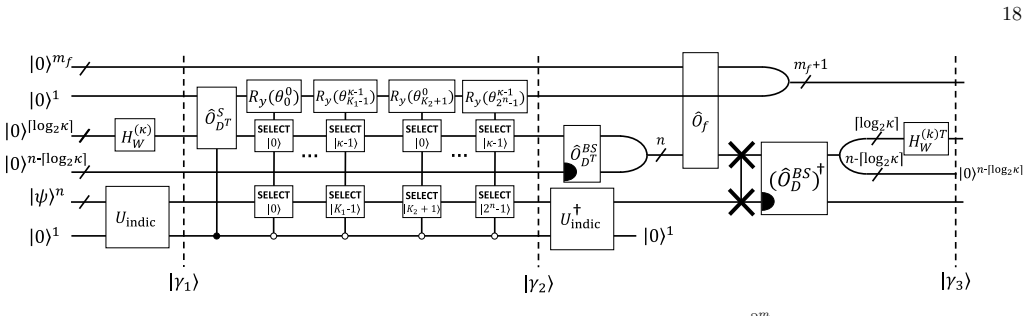
The load-bearing object is an explicit block-encoding—a unitary whose top-left block equals a scaled copy of the desired Hamiltonian—of the Hermitian Hamiltonian $H$ produced by Schrödingerisation. The encoding is assembled from three elementary oracles: (i) a banded-sparse-access oracle that converts sparse matrix indices to column indices for finite-difference matrices; (ii) a sparse-amplitude oracle that writes the normalized non-zero matrix entries into amplitudes; and (iii) an amplitude oracle, from Theorem 2, that encodes piecewise-polynomial coefficient functions $f_k$ and $v$. Robin boundary conditions are handled by an indicator unitary that flags the bulk rows, where the matrix coincides with the periodic case, and by explicitly controlled rotations for the $O(1)$ boundary-deviating rows. This block-encoding is then fed into quantum singular value transformation (Theorem 7) to realize the evolution operator $e^{-iHT}$ and, after postselection on the auxiliary registers, the desired PDE solution state.
What would settle it
Compile the Theorem 8 circuit for the 1D Robin heat equation at increasing $N=2^n$ and count CNOTs and single-qubit rotations: if the boundary-region correction requires more than $O(1)$ deviating rows per stencil, or if the total count scales faster than the stated polynomial in $2^n$ with fixed constants, the central complexity claim fails. For the d-dimensional theorem, pick a coefficient such as a non-separable function of two variables and check whether the amplitude-oracle recipe of Eq. (38) can represent it with the number of terms $M$ and polynomial degree $Q_{\rm PET}$ independent of $n$; if not, the theorem's scope is the structured-coefficient class and no further.
Extended reading notes
Core claim
The central claim is that the discretized linear PDE with Robin boundary conditions can be reduced to Hamiltonian simulation with an explicitly constructed block-encoding, so all costs are quoted in elementary gates rather than oracle queries. For the one-dimensional PDE (Eq. (1)) with $N=2^n$ grid points, Theorem 8 (informal Theorem 1) asserts that an $n$-qubit state encoding $\vec u(0)$ is mapped by an explicit gate sequence to a state proportional to $\vec u(T)$, with success probability $p_{\rm success}\sim \|\vec u(T)\|^2/\|\vec u(0)\|^2$ and gate complexity $$O\!\left((\eta\kappa n+GQ\eta n\log n)\left[T\kappa\sum_k $2^{{n p_k}}$N_{f_k}+\frac{\ln(1/\epsilon)}{\ln\left(e+\frac{\ln(1/\epsilon)}{\kappa T\sum_k $2^{{n p_k}}$N_{f_k}}\right)}\right]\right)$$ plus $O(n)$ ancillas. Theorem 9 gives the $d$-dimensional version with block-encoding cost $O(d\eta M Q_{\rm PET}GQ n\log n + d\eta\kappa n)$, linear in $d$, under the structured-coefficient assumption of Eq. (38). Numerical simulations of the 1D heat equation with Robin conditions report quantum-state fidelity above 0.99999 against a classical reference at gate counts of order $10^6$--$10^7$ for the tested 28-qubit instance.
Load-bearing premise
For the multidimensional linear-in-dimension result, every coefficient function must be built from a small number of products of one-variable piecewise-polynomial pieces, possibly fed through one low-degree polynomial; if a coefficient is genuinely multivariate, the paper notes that no efficient general encoding of such functions is known, so the linear-in-dimension bound does not follow.
Editorial extensions
If this is right
- For PDEs whose coefficients fit the structured form, the total gate count is polynomial in $N$ and linear in $d$, giving an exponential separation from classical finite-difference costs such as $O(TN^{d+g})$.
- Because Robin conditions include Neumann and Dirichlet cases, the same circuit templates cover heat, transport, and wave-type equations with variable coefficients and source terms on finite intervals or boxes.
- The quantum output is a state whose amplitudes encode the discretized solution; global quantities such as norms, expectation values, and spectral features are directly estimable, while pointwise extraction needs additional measurement rounds.
- The success probability of postselection is approximately $\|\vec u(T)\|^2/\|\vec u(0)\|^2$, so strongly damped problems pay an extra repetition overhead.
- The multidimensional advantage is conditional on the structured-coefficient assumption of Eq. (38); without it, no efficient general multivariate amplitude oracle is known, as the paper notes.
Reading between the lines
- One preprocessing step the paper does not develop: approximate a genuinely multivariate coefficient by a sum of products of univariate functions and absorb the approximation error into $\epsilon$; this would widen the class of PDEs satisfying Eq. (38).
- Because Theorem 8 avoids the structured-coefficient assumption, the most immediately testable regime is 1D and 2D with separable coefficients; a systematic comparison of actual CNOT and single-qubit rotation counts against classical FLOP counts at fixed accuracy would locate the practical crossover.
- The authors' neural-network analogy suggests that adding more LCU+PET layers expands the representable coefficient class, but each layer multiplies the block-encoding prefactor; determining the minimal layer count for a target accuracy on a given function class is a natural extension.
- The reported fidelities come from one set of simulation parameters; varying the auxiliary-register width $n_\xi$ and the phase-factor evaluation would test the robustness of the end-to-end circuit to implementation details.
Editorial analysis
A structured set of objections, weighed in public.
Referee Report
Summary. The paper proposes an explicit, oracle-free quantum algorithm for simulating linear PDEs with Robin boundary conditions, inhomogeneous terms, and variable coefficients. The method discretizes the PDE, applies Schrodingerisation to convert the non-Hermitian system into a Hamiltonian evolution, optionally adds a clock register for time-dependent coefficients, constructs block-encodings of the resulting Hamiltonian from piecewise-polynomial amplitude oracles and banded-sparse-access oracles, and then applies QSVT to realize e^{-iHt}. The main theorems (informal Theorem 1; formal Theorems 4, 6, 8, 9) give explicit gate counts and ancilla counts, and a numerical simulation of a 1D heat equation with Robin boundary conditions reports fidelity above 0.99999. The paper also extends the construction to d spatial dimensions and claims polynomial scaling in N and linear scaling in d.
Significance. If the resource estimates are correct, the paper would provide one of the more concrete, gate-counted quantum schemes for linear PDEs with general boundary conditions, avoiding the usual oracle-construction overhead and giving polynomial speedup in grid resolution and exponential-in-dimension advantage for structured coefficients. The explicit treatment of Robin boundary modifications and the inclusion of inhomogeneous terms are genuine extensions of the authors' earlier periodic-boundary work. The paper also ships a numerical demonstration on a 28-qubit simulated circuit, which is useful evidence that the core block-encoding construction works for a time-independent heat equation. However, several load-bearing points in the resource accounting and in the scope of the dimension-scaling claims need to be fixed before the advertised theorems can be accepted as stated.
major comments (4)
- [Sec. IV C / Eq. (10) / Example 1 / Thm. 1] The resource estimate in Theorem 1 and Remark 4 omits the contribution of the inhomogeneous source/boundary matrix B to ||H||_max. In Eq. (10), B = sqrt(2^n) diag{v(x_i)+v'(x_i)}, and in Example 1 the boundary correction v' scales as 1/Delta x = 2^n (e.g., v'(x0) = -7 A2/(3 Delta x)). Hence ||B|| can scale as 2^{3n/2}, and because H in Eq. (18) contains B/2 in S1 and S2, ||H||_max necessarily contains a 2^{3n/2} contribution for PDEs that include first-order or low-order derivatives. Remark 4, however, states ||H||_max ~ kappa sum_k N_{f_k} 2^{p_k n}, which only accounts for the derivative terms. The numerical test in Sec. VII uses the alternative embedding with B=I (Eq. (45)), so it does not exercise this problematic contribution. The theorem should either include the source-boundary norm in the QSVT factor or restrict the stated scope accordingly.
- [Thm. 8 / Sec. IV (Eq. 18) / Eq. (13)] Theorem 1 and Theorem 8 state results for Eq. (1) with f_k(x,t) and v(x,t) possibly time-dependent, but the block-encoding construction used in the proof (Theorem 4) is explicitly for the time-independent Hamiltonian H = S1 (x) x_xi + S2 (x) 1_xi (Eq. (18)). The clock register ps introduced in Eq. (13) for time-dependent coefficients does not appear in the 1D Hamiltonian or in the resource count of Theorem 8, and the associated ns log ns gate term is absent. Either the theorems should be restricted to time-independent coefficients, or the clock-register contribution must be included in the block-encoding construction and in the resource estimate.
- [Sec. IV F, Eq. (30)] Eq. (30) defines US1 and US2 as non-unitary linear combinations of L1, L2, X (x) OB, and Y (x) OB, and the proof of Theorem 4 refers to 'using LCU' without specifying the selector state preparation, the controlled operations, or the resulting normalization and success amplitude. Since the paper's central claim is an explicit, oracle-free gate sequence with counted resources, the LCU preparation unitaries and their gate counts need to be supplied, or a named LCU theorem must be applied with exact parameters. Without this, the claimed gate count for the block-encoding of H is not fully supported.
- [Sec. V A / Thm. 6 / Thm. 9] The claims of linear scaling in d and exponential advantage in d are conditional on the very special function class in Eq. (38), with M, QPET, G, and L_NN all O(1). The paper itself notes in Sec. V A that no efficient general multivariate amplitude oracle is known, and a generic multivariate coefficient can require exponentially many terms in the LCU decomposition. The abstract and introduction present the d-dimensional advantage without these caveats; they should be moved into the main claims, and the complexity comparison with classical solvers should explicitly display the dependence on M and QPET. As written, the dimension-scaling claim is broader than what Theorem 6 actually proves.
minor comments (5)
- [Eq. (8)] In the last row of Eq. (8), the coefficient of u_{N-1} is written as -5/2 - 7B2, but based on the boundary condition and the matrix in Eq. (9) it should be -5/2 - 7 B1 Delta x / 3; B2 only enters the inhomogeneous source term.
- [Table IV] In Table IV, the symbol M is described as the 'polynomial degree in the activation function h', but in Eq. (36) M is the number of terms in the superposition of separable functions; the polynomial degree is QPET. This should be corrected to avoid confusion.
- [Reference [3]] Reference [3] attributes 'Simulating physics with computers' to M. Pour-El and I. Richards; this is a well-known paper by R. P. Feynman and the citation appears to be incorrect.
- [Fig. 6] The caption of Fig. 6 uses both 'MSE' and 'MES' for the same quantity; the abbreviation should be unified.
- [Eq. (21)] The notation for the orthogonal component in Eq. (21), written as a superscript perpendicular followed by a ket, is nonstandard and hard to parse; a standard normalized orthogonal-state notation would improve readability.
Circularity Check
No significant circularity: the central derivation is an explicit gate-level construction with independently stated technical lemmas, not a self-referential fit.
full rationale
The central derivation is self-contained in the sense relevant to circularity. Theorem 1/8 composes explicit block-encoding constructions (Thms. 3 and 4) with the QSVT Hamiltonian-simulation theorem (Thm. 7, cited from Gilyén et al.), and the resource counts follow from gate-level implementations rather than from fitting parameters to the target output. The Robin-boundary contribution is new: the periodic constructions are modified in O(1) boundary rows through element-wise controlled Ry rotations (Eqs. 27 and 28), and the inhomogeneous term enters through an explicit matrix B = sqrt(2^n) diag{v + v'} that is block-encoded rather than assumed. Lemmas 2 and 3 and Thm. 2 are quoted from the authors' prior work, but they are technical lemmas with stated assumptions (banded sparsity, piecewise polynomial decomposition) and do not assume the present theorem; citing them is standard scientific practice and no equation in this paper reduces to its own output by construction. The numerical experiment validates the implementation against a classical finite-difference solution, rather than using the claimed complexity as evidence. The skeptic's concern that Remark 4's estimate of ||H||max omits the contribution of B is a potential correctness or complexity-accounting gap in the advertised gate count, not a circular reduction of the derivation chain.
Assumptions & free parameters
free parameters (3)
- Normalization constants N_f, N_D, N_B =
upper bounds max|f|, max|D|, max|B|
- Gaussian width sigma for clock register =
sigma -> 0 with Richardson extrapolation
- Piecewise polynomial degrees Q_g and piece counts G for f_k and v =
input-dependent representation
assumptions (6)
- domain assumption Schrodingerisation maps non-Hermitian S to Hermitian H = S1 (x) x_xi + S2 (x) 1_xi with postselection recovering u(t)
- domain assumption Piecewise continuous coefficient functions admit efficient QSP-based amplitude oracles with cost O(sum Q_g n log n)
- domain assumption Time dependence can be removed by a clock register with squeezed Gaussian state, with controllable error O(sqrt(sigma))
- standard math QSVT Hamiltonian simulation achieves optimal scaling (Thm. 7)
- domain assumption The initial condition is available as a quantum state; state preparation and measurement costs are excluded
- domain assumption Finite-difference discretization error and stability obey standard scaling, and the classical comparison cost is O(T N^{p+d})
Cite this review
Pith. "Pith review of Quantum Framework for Simulating Linear PDEs with Robin Boundary Conditions." pith.science (2026). https://pith.science/paper/MNJ4CWLF
@misc{pith2026250620478,
  author       = {Pith},
  title        = {Pith review of: Quantum Framework for Simulating Linear PDEs with Robin Boundary Conditions},
  year         = {2026},
  howpublished = {\url{https://pith.science/paper/MNJ4CWLF}},
  note         = {Machine review of arXiv:2506.20478}
}
abstract
We propose an explicit, oracle-free quantum framework for numerically simulating general linear partial differential equations (PDEs), extending previous work to incorporate (a) Robin boundary conditions - which include Neumann and Dirichlet conditions as special cases - (b) inhomogeneous terms, and (c) variable coefficients in space and time. Our approach begins with a general finite-difference discretization and applies the Schrodingerisation technique to transform the resulting system into one that admits unitary quantum evolution, enabling quantum simulation. For the Schrodinger equation corresponding to the discretized PDE, we construct an efficient block-encoding of the Hamiltonian $H$ that scales polylogarithmically with the number of grid points $N$. This encoding is compatible with quantum signal processing and allows for the implementation of the evolution operator $e^{-iHt}$. The oracle-free nature of our method permits complexity to be measured in fundamental gate units-namely, CNOT gates and single-qubit rotations-bypassing the inefficiencies of oracle queries. Consequently, the overall algorithm scales polynomially with $N$ and linearly with the spatial dimension $d$, achieving a polynomial speedup in $N$ and an exponential advantage in $d$, thereby mitigating the classical curse of dimensionality. The validity and efficiency of the proposed approach are further substantiated by numerical simulations. By explicitly defining the quantum operations and quantifying their resource requirements, our approach offers a practical alternative for numerically solving PDEs, distinct from others that rely on oracle queries and purely asymptotic scaling methods.
Figures


Figures from the paper (8 more)



Forward citations
Cited by 1 Pith paper
-
Analog photonic simulator for large-scale transport
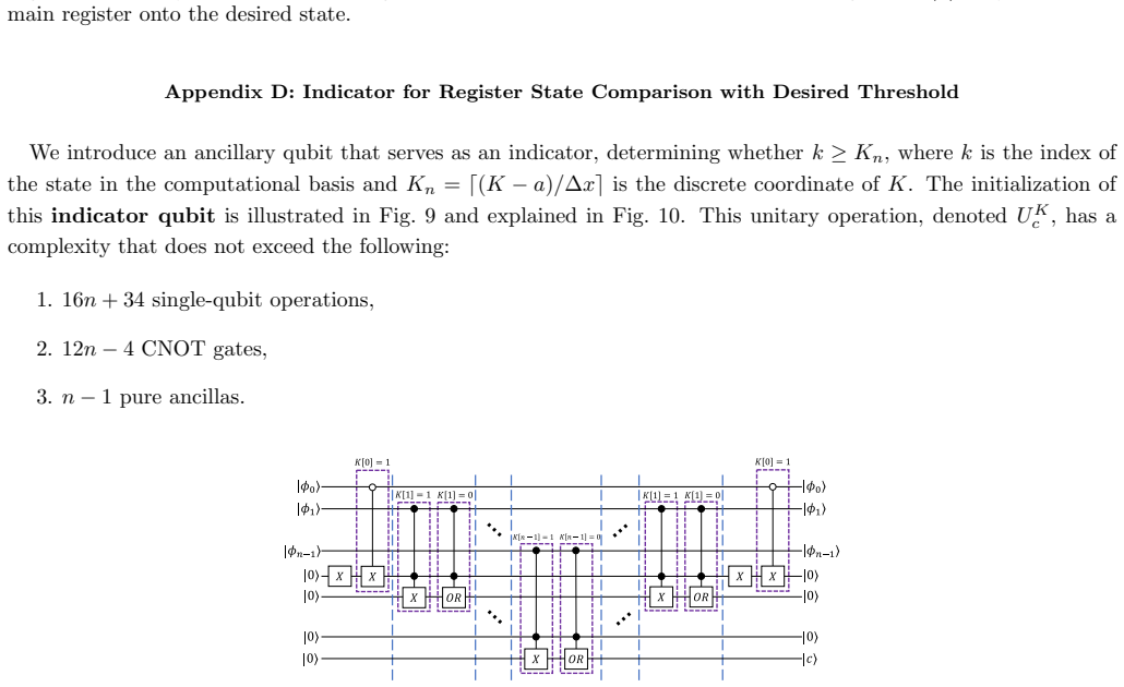
Continuous-variable photonic platform with 20,000-mode cluster state simulates advection transport equation, achieving relative errors of 0.8% and 0.92% on first- and second-order moments via homodyne readout.
Reference graph
Works this paper leans on
-
[1]
(2l + 1)(32n − 48) single-qubit operations
-
[2]
25 · 2ln − 36 · 2l + 32n − 48 CNOT gates
-
[3]
n − 1 pure ancilla qubits. Remark 2 Note that the Banded-sparse-access-oracle with the largest diagonal sparsity index smax = 7 can be con- structed for matrix A from Example 1; thus, the matrix contains 7 diagonals with non-zero elements (including 2 additional diagonals arising from boundary effects). Later on we use Banded-sparse-access-oracles to swit...
-
[4]
2l single-qubit operations
-
[5]
2l CNOT gates. Remark 3 This Sparse-amplitude-oracle is particularly used for encoding higher-order derivative operators with peri- odic boundary conditions, such as ∂m/∂xm arising from finite-difference formulas(see Table. I); since these matrices maintain an identical banded pattern across all rows, the oracle construction remains valid for arbitrary de...
-
[6]
O(PG g=1 Qgn log n) quantum gates
-
[7]
n − 1 pure ancillas (see Definition 2). Applying Thm. 2 to the function v(x) + v′(x) enables us to construct a ( NB, ⌈log2 n⌉ + ⌈log2 Gv⌉ + 3, 0)-block- encoding of the matrix B, denoted by ˆOB. Here, the normalization factor satisfies NB ∼ √ 2n maxx∈[a,b] v(x), as discussed in Eq. (10) and Definition 3. Similarly, we can construct ˆOf which is a ( Nf , ⌈...
-
[8]
O PG g=1 Qgn log n + 2ln quantum gates
Show all 82 references
-
[9]
The following equation clarifies the structure of Fig
2 n − l pure ancillas. The following equation clarifies the structure of Fig. 2. As input, we use an arbitrary quantum state |ψ⟩n =P2n−1 j=0 σj |j⟩n. The index s refers to the diagonal sparsity index (see Lemma 1), and F (Ak, i) denotes the set of column indices corresponding ...
-
[10]
Note, we always can include zeros in the set of non-zero elements, so we now use the diagonal sparsity of matrix A smax = κ, see Remark 2
n pure ancillas. Note, we always can include zeros in the set of non-zero elements, so we now use the diagonal sparsity of matrix A smax = κ, see Remark 2. Lastly, let us consider the boundary part of the discretized derivative operator D ∼ ∂m ∂xm from the Eq. (6) for Robin 17...
-
[11]
O PG g=1 Qgn log n + κ (K1 + 2n − K2)| {z } the number of deviating lines n quantum gates
-
[12]
2 n pure ancillas. The total number of deviating indices, K1 + 2n − K2, can be safely assumed to be O(1) as it depends linearly on the degree of accuracy of the finite-difference scheme used, which is a small number [35, 36]. Thus, we can prove the following Theorem. Theorem 3...
-
[13]
O PG g=1 Qgn log n + κn quantum gates
-
[14]
2n pure ancillas. |γ1⟩ = 1 ND √κ X s=0,...,κ−1 0≤j<K1∪K2<j<2n σj |0⟩mf |0⟩1 |s⟩⌈log2 κ⌉ |0⟩n−⌈log2 κ⌉ |j⟩n |0⟩1 + 1√κ X s=0,...,κ−1 K1≤j≤K2 σj |0⟩mf |0⟩1 |s⟩⌈log2 κ⌉ |0⟩n−⌈log2 κ⌉ |j⟩n |1⟩1 ; |γ2⟩ = 1 ND √κ X s=0,...,κ−1 0≤j<K1∪K2<j<2n (DT )(s) j σj |0⟩mf |0⟩1 |s⟩⌈log2 κ⌉ |0⟩n...
-
[15]
O(nξ log nξ) quantum gates
-
[16]
Thus, the following theorem summarizes the results of this section
⌈log2 nξ⌉ −1 pure ancillas. Thus, the following theorem summarizes the results of this section. Theorem 4 (One-dimensional block-encoding) Let H be a 2n+1 · 2nξ × 2n+1 · 2nξ Hermitian matrix with sparsity κ. The matrix H represents the Hamiltonian of an n + nξ-qubit system, go...
-
[17]
O(PGv g=0 Qv gn log n + Pη−1 k=0 κkn + PGfk g=0 Qfk g n log n + nξ log nξ) quantum gates,
-
[18]
2n + 2 pure ancillas, where κk is a sparsity of Ak; Gv and Gfk are the number of pieces in v(x), fk(x) respectively; Qfk g , and Qv g are the polynomial degrees, see Thm. 2. We clarify the key notations in Table II. Proof. This entire section provides a step-by-step explanatio...
-
[19]
Block-encoding for d-D Hamiltonian Let us now consider the rest part of the Eq
+ tanhr · x1x2 1 Quantum optics, continuous- variable quantum states Interacting field kernel exp −λx2 1x2 2 2 Scalar quantum fields, ϕ4 theory Radial potential well χ[0,R]( p x2 + y2) 1 Radially symmetric traps or dots Step function barrier V0 · χ[x1,x2](x) 1 Potential wells,...
-
[20]
O(M QPETGQ(dn log n + ns log ns) + nξ log nξ + dηκn) quantum gates,
-
[21]
The key notations are given in Table IV
O(n) pure ancillas. The key notations are given in Table IV. Proof. The overall idea repeats the proof of Thm. 4 with A(d) instead of A. The construction of A(d) is described above in this Section. The main difficulty in the multi-dimensional case is the block-encoding of B(d)...
-
[22]
Ω(t, ϵ) uses of UH or its inverse
-
[23]
1 use of controlled-U or its inverse
-
[24]
Ω(αt, ϵ)(16a + 50) + 4 one-qubit gates
-
[25]
Ω(αt, ϵ)(12a + 38) CNOT gates
-
[26]
Ω(αt, ϵ) is implicitly defined through inequality for the truncation parameter g ≥ Ω(αt, ϵ) 1.07√g αet 2g g ≤ ϵ
O(n) ancilla qubits. Ω(αt, ϵ) is implicitly defined through inequality for the truncation parameter g ≥ Ω(αt, ϵ) 1.07√g αet 2g g ≤ ϵ. 27 The inequality determines scaling of the algorithm (Lemma 59 from [24]) Ω(αt, ϵ) = O αt + ln(1/ϵ) ln e + ln(1/ϵ) αt The following two...
-
[27]
O( κ||H||maxt + ln(1/ϵ) ln(e+ ln(1/ϵ) κ||H||max t ) · PGv g=0 Qv gn log n + Pη−1 k=0 κkn + PGfk g=0 Qfk g n log n + nξ log nξ quantum gates,
-
[28]
2n + 3 pure ancillas, where κk is a sparsity of Ak; Gv and Gfk are the number of pieces in v(x), fk(x) respectively; Qfk g , and Qv g are the polynomial degrees, see Thm. 2. We clarify the key notations in Table II. Proof. Applying Optimal block-Hamiltonian simulation (Thm. 7)...
-
[29]
O( κ||H||maxt + ln(1/ϵ) ln(e+ ln(1/ϵ) κ||H||max t ) · (ηM QPETGQ(dn log n + ns log ns) + nξ log nξ + dηκn) quantum gates,
-
[30]
O(n) pure ancillas, We clarify the key notations in Table IV. 28 Corollary 1 (Postselection)Consequently, if we have a black-box quantum access to the initial condition ⃗ u(t = 0), then we can get the quantum state ⃗ u(t)/||⃗ u(t)|| with additional resources for QF T−1: O(n2 ξ...
-
[31]
Guseynov, X
N. Guseynov, X. Huang, and N. Liu, Efficient explicit gate construction of block-encoding for hamiltonians needed for simulating partial differential equations, Phys. Rev. Res. , (2025)
2025
-
[32]
L. C. Evans, Partial differential equations , Vol. 19 (American Mathematical Society, 2022)
2022
-
[33]
Pour-El and I
M. Pour-El and I. Richards, Simulating physics with computers, International Journal of Theoretical Physics 21, 553 (1982)
1982
-
[34]
R. B. Laughlin and D. Pines, The theory of everything, Proceedings of the national academy of sciences 97, 28 (2000)
2000
-
[35]
P. C. Costa, S. Jordan, and A. Ostrander, Quantum algorithm for simulating the wave equation, Physical Review A 99, 012323 (2019)
2019
-
[36]
Gaitan, Finding flows of a navier–stokes fluid through quantum computing, npj Quantum Information 6, 61 (2020)
F. Gaitan, Finding flows of a navier–stokes fluid through quantum computing, npj Quantum Information 6, 61 (2020)
2020
-
[37]
S. Jin, N. Liu, and Y. Yu, Time complexity analysis of quantum algorithms via linear representations for nonlinear ordinary and partial differential equations, Journal of Computational Physics 487, 112149 (2023)
2023
-
[38]
Linden, A
N. Linden, A. Montanaro, and C. Shao, Quantum vs. classical algorithms for solving the heat equation, Communications in Mathematical Physics 395, 601 (2022)
2022
-
[39]
Y. Sato, R. Kondo, I. Hamamura, T. Onodera, and N. Yamamoto, Hamiltonian simulation for time-evolving partial differential equation by scalable quantum circuits, arXiv preprint arXiv:2402.18398 (2024)
2024 arXiv
-
[40]
Stamatopoulos, D
N. Stamatopoulos, D. J. Egger, Y. Sun, C. Zoufal, R. Iten, N. Shen, and S. Woerner, Option pricing using quantum computers, Quantum 4, 291 (2020)
2020
-
[41]
Gonzalez-Conde, ´A
J. Gonzalez-Conde, ´A. Rodr ´ ıguez-Rozas, E. Solano, and M. Sanz, Efficient hamiltonian simulation for solving option price dynamics, Physical Review Research 5, 043220 (2023). 33
2023
-
[42]
L. K. Grover, A fast quantum mechanical algorithm for database search, in Proceedings of the twenty-eighth annual ACM symposium on Theory of computing (1996) pp. 212–219
1996
-
[43]
M. A. Nielsen and I. L. Chuang, Quantum Computation and Quantum Information: 10th Anniversary Edition (Cambridge University Press, 2011)
2011
-
[44]
A. W. Harrow, A. Hassidim, and S. Lloyd, Quantum algorithm for linear systems of equations, Phys. Rev. Lett. 103, 150502 (2009)
2009
-
[45]
D. W. Berry, A. M. Childs, and R. Kothari, Hamiltonian simulation with nearly optimal dependence on all parameters, in 2015 IEEE 56th annual symposium on foundations of computer science (IEEE, 2015) pp. 792–809
2015
-
[46]
P. Rall, C. Wang, and P. Wocjan, Thermal state preparation via rounding promises, Quantum 7, 1132 (2023)
2023
-
[47]
C. M. Dawson and M. A. Nielsen, The solovay-kitaev algorithm, arXiv preprint quant-ph/0505030 (2005)
2005 arXiv
-
[49]
S. Jin, N. Liu, and Y. Yu, Quantum simulation of partial differential equations: Applications and detailed analysis, Physical Review A 108, 032603 (2023)
2023
-
[50]
Jin and N
S. Jin and N. Liu, Analog quantum simulation of partial differential equations, Quantum Science and Technology 9, 035047 (2024)
2024
-
[51]
Y. Cao, S. Jin, and N. Liu, Quantum simulation for time-dependent hamiltonians–with applications to non-autonomous ordinary and partial differential equations, Journal of Physics A: Mathematical and Theoretical (2023)
2023
-
[52]
Jin and N
S. Jin and N. Liu, Quantum simulation of discrete linear dynamical systems and simple iterative methods in linear algebra, Proceedings of the Royal Society A 480, 20230370 (2024)
2024
-
[53]
Y. Cao, S. Jin, and N. Liu, A unifying framework for quantum simulation algorithms for time-dependent hamiltonian dynamics, arXiv preprint arXiv:2411.03180 (2024)
2024 arXiv
-
[54]
Gily´ en, Y
A. Gily´ en, Y. Su, G. H. Low, and N. Wiebe, Quantum singular value transformation and beyond: exponential improvements for quantum matrix arithmetics, in Proceedings of the 51st Annual ACM SIGACT Symposium on Theory of Computing (2019) pp. 193–204
2019
-
[55]
G. H. Low and I. L. Chuang, Optimal hamiltonian simulation by quantum signal processing, Physical review letters 118, 010501 (2017)
2017
-
[56]
R. J. LeVeque, Finite difference methods for ordinary and partial differential equations: steady-state and time-dependent problems (SIAM, 2007)
2007
-
[57]
Kharazi, A
T. Kharazi, A. M. Alkadri, J.-P. Liu, K. K. Mandadapu, and K. B. Whaley, Explicit block encodings of boundary value problems for many-body elliptic operators, Quantum 9, 1764 (2025)
2025
-
[58]
D. W. Berry, A. M. Childs, R. Cleve, R. Kothari, and R. D. Somma, Exponential improvement in precision for simulating sparse hamiltonians, in Proceedings of the forty-sixth annual ACM symposium on Theory of computing (2014) pp. 283–292
2014
-
[59]
Mu˜ noz-Coreas and H
E. Mu˜ noz-Coreas and H. Thapliyal, T-count and qubit optimized quantum circuit design of the non-restoring square root algorithm, ACM Journal on Emerging Technologies in Computing Systems (JETC) 14, 1 (2018)
2018
-
[60]
H¨ aner, M
T. H¨ aner, M. Roetteler, and K. M. Svore, Optimizing quantum circuits for arithmetic, arXiv preprint arXiv:1805.12445 (2018)
2018 arXiv
-
[61]
J. Hu, S. Jin, N. Liu, and L. Zhang, Quantum circuits for partial differential equations via schr¨ odingerisation, Quantum 8, 1563 (2024)
2024
-
[62]
Y. Cao, A. Papageorgiou, I. Petras, J. Traub, and S. Kais, Quantum algorithm and circuit design solving the poisson equation, New Journal of Physics 15, 013021 (2013)
2013
-
[63]
S. Jin, N. Liu, and C. Ma, On schr¨ odingerization based quantum algorithms for linear dynamical systems with inhomoge- neous terms, arXiv preprint arXiv:2402.14696 (2024)
2024 arXiv
-
[64]
S. Jin, N. Liu, C. Ma, and Y. Yu, On the schr¨ odingerization method for linear non-unitary dynamics with optimal dependence on matrix queries, arXiv preprint arXiv:2505.00370 (2025)
2025
-
[65]
O. C. Zienkiewicz, R. L. Taylor, and J. Z. Zhu, The finite element method: its basis and fundamentals (Elsevier, 2005)
2005
-
[66]
M. N. ¨Ozi¸ sik, H. R. Orlande, M. J. Cola¸ co, and R. M. Cotta,Finite difference methods in heat transfer (CRC press, 2017)
2017
-
[67]
Guseynov and N
N. Guseynov and N. Liu, Efficient explicit circuit for quantum state preparation of piece-wise continuous functions, arXiv preprint arXiv:2411.01131 (2024)
2024
-
[68]
Shukla and P
A. Shukla and P. Vedula, An efficient quantum algorithm for preparation of uniform quantum superposition states, Quan- tum Information Processing 23, 38 (2024). 34
2024
-
[69]
Z. M. Rossi and I. L. Chuang, Multivariable quantum signal processing (m-qsp): prophecies of the two-headed oracle, Quantum 6, 811 (2022)
2022
-
[70]
Samek, G
W. Samek, G. Montavon, S. Lapuschkin, C. J. Anders, and K.-R. M¨ uller, Explaining deep neural networks and beyond: A review of methods and applications, Proceedings of the IEEE 109, 247 (2021)
2021
-
[71]
A. M. Dalzell, S. McArdle, M. Berta, P. Bienias, C.-F. Chen, A. Gily´ en, C. T. Hann, M. J. Kastoryano, E. T. Khabi- boulline, A. Kubica, et al. , Quantum algorithms: A survey of applications and end-to-end complexities, arXiv preprint arXiv:2310.03011 (2023)
2023 arXiv
-
[72]
S. Aaronson, Shadow tomography of quantum states, in Proceedings of the 50th Annual ACM SIGACT Symposium on Theory of Computing , STOC 2018 (Association for Computing Machinery, New York, NY, USA, 2018) p. 325–338
2018
-
[73]
Huang, R
H.-Y. Huang, R. Kueng, and J. Preskill, Predicting many properties of a quantum system from very few measurements, Nature Physics 16, 1050 (2020)
2020
-
[74]
Y. Dong, X. Meng, K. B. Whaley, and L. Lin, Efficient phase-factor evaluation in quantum signal processing, Physical Review A 103, 042419 (2021)
2021
-
[75]
https://qsppack.gitbook.io/qsppack
-
[76]
Huang and N
X. Huang and N. Guseynov, Hamiltonian simulation of 1d heat equation with robin boundary conditions, https://github. com/XiajieHuang/Hamiltonian-Simulation-of-1D-Heat-Equation-with-Robin-Boundary-Conditions (2025)
2025
-
[77]
S. Jin, N. Liu, and Y. Yu, Quantum simulation of partial differential equations via schr¨ odingerization, Physical Review Letters 133, 230602 (2024)
2024
-
[78]
Gautschi, Numerical analysis (Springer Science & Business Media, 2011)
W. Gautschi, Numerical analysis (Springer Science & Business Media, 2011)
2011
-
[79]
Kress, Numerical analysis, Vol
R. Kress, Numerical analysis, Vol. 181 (Springer Science & Business Media, 2012)
2012
-
[80]
Saad, Iterative methods for sparse linear systems (SIAM, 2003)
Y. Saad, Iterative methods for sparse linear systems (SIAM, 2003). Appendix A: The complexity analysis for classical methods In this section, we analyze the computational complexity for classical methods, including explicit schemes such as the forward Euler method, and implici...
2003
-
[81]
16 n + 34 single-qubit operations,
-
[82]
12 n − 4 CNOT gates,
-
[83]
n − 1 pure ancillas. Fig. 9: Circuit design for initializing the indicator qubit. This circuit functions similarly to a classical comparator, comparing the computational basis state in the upper register with K, and setting the last qubit to |c⟩ = |1⟩ if ϕ ≥ Kn. The circuit ut...
Reviewed August 6, 2026 · model on record in the stance chip above.
Discussion (0). Sign in to comment.