REVIEW 4 major objections 6 minor 79 references
Consequences of Non-Gaussian Instrumental Noise in Perturbed Nulling Interferometers
T0 review · 4 major / 6 minor · reviewed 2026-08-06 · deepseek-v4-flash
Pith's one-line read A dual Bracewell nuller's differential output cannot have Gaussian noise: the phase–amplitude cross term is a product of Gaussians whose true distribution is an iterated Bessel convolution.
desk verdict Non-Gaussian noise in dual Bracewell nullers is real; the IMB model is a useful semi-empirical fit, but the analytic proof doesn't cover the matched-filter case and the tail correction is extrapolated far beyond the fitted range. read the letter →
The pith
A machine-rendered reading of the paper's core claim, the machinery that carries it, and where it could break.
The reading
What carries the argument
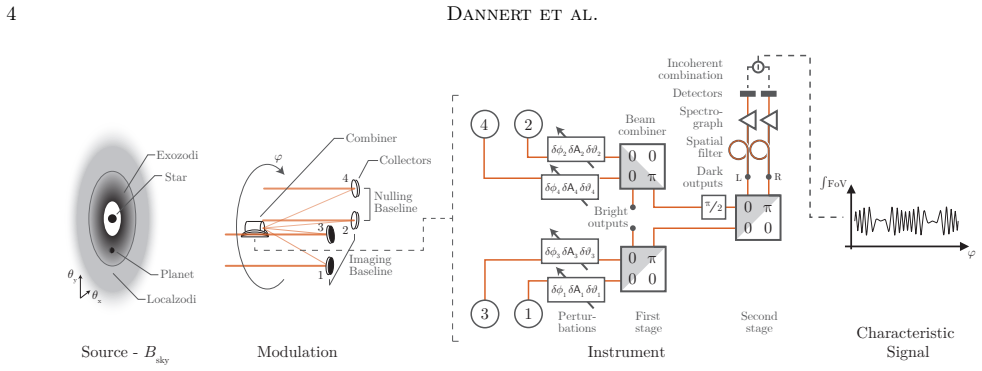
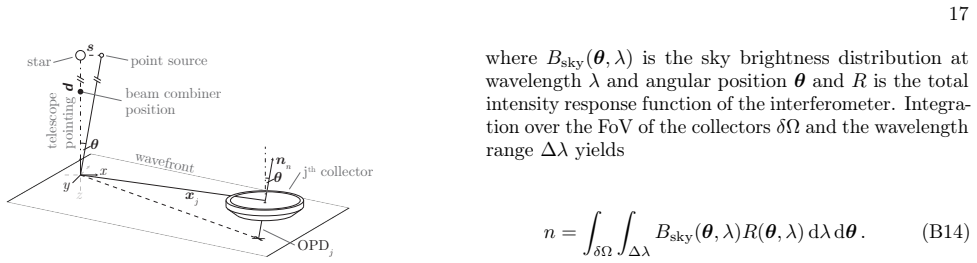
The load-bearing objects are: (1) the van Cittert–Zernike instrument model of Equation (1), which writes the photon rate as Fourier transforms of the sky brightness evaluated at the array baselines; (2) the second-order Taylor expansion of Equation (3), in which identical perturbations in the two dark outputs cancel all symmetric terms and leave only the first-order phase term and the mixed phase–amplitude cross term; (3) the IMB probability density of Equation (28), obtained from the characteristic function of the $K_0$-Bessel product-of-Gaussians distribution via the convolution theorem; and (4) the matched-filter test statistic of Equation (16), evaluated in Fourier space using the pink-noise power spectral density of Equation (19). The mechanism is that a product of Gaussian perturbations is heavy-tailed, temporal correlations reduce the effective number of independent samples from $N$ to the fitted $\nu=36$, and mixing this IMB component with the Gaussian approximation of photon noise shifts the critical values of the test statistic away from the Gaussian ones.
What would settle it
Generate $10^8$ planet-free matched-filter outputs from the reference dual Bracewell model with Gaussian pink-noise perturbations and count realizations exceeding the Gaussian $5\sigma$ threshold: the paper's IMB model predicts a false-positive rate above $2.9\times10^{-7}$, so an observed rate indistinguishable from the Gaussian value would falsify the central claim.
Extended reading notes
Core claim
The paper's central claim is that the null-hypothesis distribution of the matched-filter output of a dual Bracewell nulling interferometer is non-Gaussian and follows an iteratively convolved Bessel distribution. After subtraction of the two dark outputs, the Taylor-expanded differential rate of Equation (3) contains only a first-order phase term and a second-order mixed term $\delta A^T (\partial^2 n/\partial A\partial\phi)\delta\phi$; this mixed term is a quadratic form in two Gaussian vectors, so the distribution of each frequency component is a modified Bessel function $K_0$, and the sum over many independent modes is the IMB distribution of Equation (28). The paper calibrates the shape parameter by drawing $10^8$ correlated time series from its instrument model and finds $\nu=36$ for the reference setup, then bootstraps $10^{10}$ realizations of the test statistic to build a lookup table for the correction factor $T_N/T_\alpha$. The consequence is that quoting a Gaussian S/N with $5\sigma$ or $7\sigma$ thresholds understates the true false-positive rate; for the reference setup a nominal $7.90\sigma$ detection at $10\,\mu$m corresponds to about 6% lower significance, and the paper quantifies this with the $T_N/T_\alpha$ correction.
Load-bearing premise
The argument rests on the inputs being zero-mean Gaussian pink-noise perturbations with the power spectral density of Equation (19), and on the two dark outputs experiencing identical perturbations so common-mode terms cancel; Section 5.4 concedes that the real perturbation distribution is probably more complicated, and if either assumption fails the specific Bessel form with $\nu=36$ does not apply, though heavy-tailed non-Gaussianity would likely survive.
Editorial extensions
If this is right
- Standard Gaussian S/N thresholds in nulling interferometry set the false-positive rate too low; for the reference Earth-twin setup the nominal $7.90\sigma$ detection in the $10\,\mu$m channel is about $6\%$ less significant, equivalent to roughly $14\%$ more integration time.
- The correction factor $T_N/T_\alpha$ collapses onto the ratio $\sigma_{\mathrm{IMB}}/\sigma_N$, so a lookup table calibrated for one shape parameter $\nu$ can be reused across different noise strengths without new Monte Carlo runs.
- In the reference case the second-order phase–amplitude term dominates the first-order phase term, so the systematic noise in the differential output is set by the imaging baseline rather than the nulling baseline.
- The non-Gaussian correction is negligible for broadband Earth-twin detection, where per-channel significances are low, but it matters for high-significance single-wavelength characterization, where $T_N/T_\alpha\approx 0.92$ at $10\,\mu$m.
- Equation (16) evaluates a multi-day observation's significance in seconds from perturbation power spectra, making the correction cheap enough to embed in exoplanet yield simulations.
Reading between the lines
- Beyond the paper, if the input perturbations are non-Gaussian or common-mode rejection between the two dark outputs is imperfect, the specific Bessel form and the fitted $\nu=36$ will not hold; the paper itself notes in Section 5.4 that the true perturbation distribution is likely more complicated, and a testbench measurement of the null distribution could act as a diagnostic of second-order pertu
- The fitted degrees of freedom $\nu$ probably equals the effective number of independent samples set by the overlap of the perturbation PSD with the planet-modulation template; if so, $\nu$ could be predicted analytically from the quantities in Equation (15) rather than fitted from $10^8$ simulated observations.
- Because spectral correlations can be used to calibrate systematic noise, the single-channel correction is likely an upper bound for broadband yield calculations; the main mission-design impact would then be on per-channel spectroscopy rather than on overall detection rates.
- The same matched-filter IMB machinery may transfer to single-aperture high-contrast imaging, where speckle noise is also known to be non-Gaussian, potentially giving a common false-positive-control framework across direct-imaging architectures.
Signed reviews
Editorial analysis
A structured set of objections, weighed in public.
Referee Report
Summary. The paper considers a dual Bracewell nulling interferometer subject to Gaussian pink-noise perturbations in phase and amplitude. Starting from the Lay (2004) Taylor-expanded instrument response, it derives the differential-output photon rate, constructs a matched-filter test statistic, and provides a semi-analytical frequency-domain expression for its variance. The central statistical claim is that the second-order phase-amplitude term in Equation (3) is a product of Gaussian perturbations, so the systematic noise in the differential output cannot be Gaussian; the paper derives an 'iterative-convolved modified Bessel' (IMB) distribution for the white-noise case, fits its degrees-of-freedom parameter to correlated pink-noise simulations (finding ν=36), bootstraps the test statistic, and constructs a lookup table correcting Gaussian-significance thresholds (TN) to the true thresholds (Tα). A reference-case noise budget for an Earth-twin observation yields TN=7.90 versus Tα=8.42, i.e., a ~6% overestimate of significance if Gaussianity is assumed. The method is implemented in the public package InLIFEsim, and the analytical response is cross-validated against LIFEsim in Appendix B.3.
Significance. The question addressed is important: nulling interferometry performance predictions for mission concepts such as LIFE typically assume Gaussian noise, and if systematic instrumental noise is genuinely heavier-tailed, detection thresholds and yield estimates could be biased. The paper contributes a computationally efficient semi-analytical instrument model, a public codebase, and a concrete quantitative recipe (variance formula plus correction factor) that can be integrated into yield simulations. The core observation that a product of Gaussian perturbations is non-Gaussian is robust, and the historical context (Mennesson et al. 2010; Hanot et al. 2011; Bonse et al. 2023) supports the relevance of non-Gaussian noise in high-contrast instrumentation. The paper is also commendably explicit about many of its limitations in Section 5.4. However, the specific analytical identification of the matched-filter noise as IMB-distributed in the realistic template-weighted, correlated case is not established, and the quantitative tail correction rests on an unvalidated extrapolation; these issues are load-bearing for the paper's headline claims.
major comments (4)
- [§4.1, Eqs. (25)–(27)] The characteristic-function argument proves that the unweighted sum w' = Σ_i x_i y_i is IMB-distributed, but the extension to the weighted sum w = Σ_i x_i y_i η_i is not valid for a time-varying template. The characteristic function is φ_w(ω) = ∏_i [1 + (2π σ_x σ_y η_i ω)^2]^{-1/2}, which reduces to a single IMB characteristic function only when all η_i are equal. The text after Eq. (27) states that 'as η is a constant vector, PDF_w' and PDF_w differ only up to a constant,' but the actual planet template η is strongly time-dependent (Fig. 5). The claimed identification of the matched-filter noise distribution as a single IMB distribution is therefore not proven for the realistic case.
- [§4.2, Fig. 3, Table 2] The numerical calibration of ν=36 uses 10^8 simulated template-matched noise values, and the reported QQ R²=0.9992 is dominated by central quantiles. The resulting lookup table is applied in Table 2 at TN=7.90, corresponding to α=3.6×10^-15, far beyond the 10^8-sample range. The logistic extrapolation in Appendix D is used without any uncertainty propagation from the ν fit or from the tail extrapolation. Consequently, the quantitative TN/Tα correction factor is an empirical approximation whose tail accuracy is unvalidated, and the statement that the correction is ~6% at TN=7.9 is not supported with confidence bounds.
- [§4.1 and Eq. (18)] The analytical derivation treats w = Σ_i x_i y_i η_i, a single-index sum, whereas the actual second-order systematic noise in Eq. (18) is a double sum Σ_{i,j} (∂²n/∂A_i∂φ_j) δA_i δφ_j, with the mixed Hessian in Eq. (B43) non-diagonal. The reduction of this quadratic form to the simple product-sum model of §4.1 is not demonstrated. Since the fitted ν in §4.2 is calibrated on the full correlated model, a good central fit can mask this misspecification; the tail behavior, where the lookup table is used, is precisely where such misspecification would be most severe.
- [Abstract and §5.4] The abstract claims that the paper derives 'the true noise distribution of the differential output' and that it 'follows iterative convolutions of Bessel functions.' Section 5.4 itself lists major caveats: the actual perturbation distribution is likely far more complicated than Gaussian pink noise, the lookup table is not universal and depends on the target and instrument configuration, spectral correlations are ignored, and the matched filter assumes a priori knowledge of the planet position. The conclusions should be reframed as applying to the specific Gaussian-pink-noise, single-wavelength, perfectly common-mode-rejected model, and the 'true distribution' language should be softened accordingly.
minor comments (6)
- [Eq. (25)] The characteristic function of the normalized K0 density in Eq. (23) should satisfy φ_ui(0)=1, but the expression in Eq. (25) gives φ_ui(0)=π σx σy. The final density is renormalized in Eq. (28), but the notation is inconsistent and should be clarified.
- [Throughout] The manuscript contains numerous unresolved cross-reference placeholders such as '?? section 2', '?? section 3', and '?? section 5'; these should be fixed before submission.
- [Fig. 3] The y-axis of the left panel appears garbled ('10□6' instead of a power-of-ten label), and the legend entries for the QQ plot do not clearly map to the plotted lines and R² values.
- [§4.2] The statement that 'a pure PDF-based comparison is not sufficient' is followed by a QQ analysis, but the QQ coefficient of determination is also dominated by central quantiles; specifying the quantile range used or adding a tail-weighted diagnostic would be more informative for the extreme-event behavior.
- [Eq. (2) and Appendix B.4] The remainder term is denoted R_2 but the text describes it as 'the third order remainder'; the indexing should be made consistent.
- [§4.3, Eq. (30)] The sum N(0,σ_N) + IMB(0,σ_IMB,ν) is not itself IMB-distributed; the text should state explicitly that the distribution of the test statistic T is obtained numerically by sampling from this sum, not by a closed-form convolution.
Circularity Check
Correlated-noise IMB and the TN/Tα detection correction reduce to a fit of ν; the white-noise non-Gaussianity claim is independently grounded.
-
fitted input called prediction
[Section 4.2 (Figure 3), Section 6 summary step 4b; applied in Section 4.3 and Table 2]
"The noise samples produced in 3c) are used to numerically fit ν. This results in an analytical formulation of the noise distribution PDFIMB(ν, µ, σ). ... For the given setup, the best fit is found for ν = 36 with R2 = 0.9992 (see Figure 3)."
The correlated-noise IMB form is not derived; the shape parameter ν is fitted to 10^8 synthetic matched-filter outputs generated by the paper's own instrument model. That fitted PDF_IMB(ν=36) is then used to bootstrap the test statistic and build the TN/Tα lookup table, from which Table 2's claimed α=3.6×10^-15 at TN=7.90 is read. The quantitative 'semi-analytical prediction of detection performance' is therefore a deterministic function of the fitted ν and of the assumed IMB family, not an independent first-principles result. The tail at α~10^-15 is extrapolated beyond the 10^8 samples used for the fit via the IMB model and logistic fits (Appendix D), so the headline correction is forced by the fit rather than by data or derivation.
full rationale
The core mathematical claim that the second-order phase-amplitude term δA·δφ is non-Gaussian for Gaussian inputs is independently derived and correct. The white-noise IMB derivation (Section 4.1) is a valid result for unweighted sums of such products. However, the paper's own pipeline for the reference correlated case does not derive the IMB form; Section 4.2 fits ν to 10^8 samples generated by the paper's instrument model, and Section 4.3 uses that fitted distribution to produce the test-statistic distribution and the TN/Tα correction. The quantitative detection-correction prediction therefore reduces, by the paper's own pipeline, to a fitted parameter. A separate correctness risk, not itself circularity, is that the proof's extension to the matched filter assumes η is a constant vector (Section 4.1), while the actual planet template varies strongly with time (Figure 5); this undermines the claim that the template-weighted noise is exactly IMB, but the paper's numerical ν fit and logistic tail extrapolation stand in for that missing derivation. No load-bearing self-citation or imported uniqueness theorem was found; the self-citations to Dannert et al. (2022) and Bonse et al. (2023) are contextual and not load-bearing.
Assumptions & free parameters
free parameters (4)
- IMB degrees of freedom nu =
36 for the reference case
- Phase perturbation rms =
0.0013 rad with 1/f PSD
- Relative amplitude perturbation rms =
0.0013 with 1/f PSD
- Polarization perturbation rms =
0.0013 rad with 1/f PSD
assumptions (8)
- domain assumption Input phase and amplitude perturbations follow zero-mean Gaussian pink noise with PSD defined in Equation (19).
- domain assumption Perturbations in the two dark outputs are identical (delta_beta_minus = 0).
- domain assumption The beam combiner is linear and single-mode spatial filtering has no cross-talk between spatial modes.
- domain assumption Random and systematic noise contributions are independent, and the Fourier modes of the noise are independent.
- domain assumption Random photon noise is approximated as Gaussian in the bootstrap.
- domain assumption The second-order Taylor expansion of the photon rate is sufficient, with remainder below 0.4 percent for reference perturbations.
- standard math Standard results: the product of independent Gaussians follows a K0 Bessel distribution, Plancherel theorem, and the central limit theorem.
- domain assumption The matched filter template is known a priori, meaning the planet position is known before the measurement.
invented entities (1)
-
IMB distribution (iterative-convolved modified Bessel noise distribution)
Cite this review
Pith. "Pith review of Consequences of Non-Gaussian Instrumental Noise in Perturbed Nulling Interferometers." pith.science (2026). https://pith.science/paper/RFPXJAQ5
@misc{pith2026250620653,
  author       = {Pith},
  title        = {Pith review of: Consequences of Non-Gaussian Instrumental Noise in Perturbed Nulling Interferometers},
  year         = {2026},
  howpublished = {\url{https://pith.science/paper/RFPXJAQ5}},
  note         = {Machine review of arXiv:2506.20653}
}
read the original abstract
With the astrophysics community working towards the first observations and characterizations of Earth-like exoplanets, interest in space-based nulling interferometry has been renewed. This technique promises unique scientific and technical advantages by enabling direct mid-infrared observations. However, concept studies of nulling interferometers often overlook the impact of systematic noise caused by instrument perturbations. Earlier research introduced analytical and numerical models to address instrumental noise and, building on these results, we reproduce key simulations and report that the noise in the differential output of nulling interferometers follows a non-Gaussian distribution. The presence of non-Gaussian noise challenges the validity of classical hypothesis tests in detection performance estimates, as their reliance on Gaussian assumptions leads to overconfidence in detection thresholds. For the first time, we derive the true noise distribution of the differential output of a dual Bracewell nulling interferometer, demonstrating that it follows iterative convolutions of Bessel functions. Understanding this noise distribution enables a refined formulation of hypothesis testing in nulling interferometry, leading to a semi-analytical prediction of detection performance. This computationally efficient instrument model, implemented in a publicly available codebase, is designed for integration into science yield predictions for nulling interferometry mission concepts. It will play a key role in refining key mission parameters for the Large Interferometer For Exoplanets (LIFE).
Figures


Figures from the paper (7 more)




Reference graph
Works this paper leans on
-
[1]
Alei, E., Quanz, S. P., Konrad, B. S., et al. 2024, A&A, 689, A245, doi: 10.1051/0004-6361/202450320
-
[2]
2023, Astrobiology, 23, 183–194, doi: 10.1089/ast.2022.0010
Angerhausen, D., Ottiger, M., Dannert, F., et al. 2023, Astrobiology, 23, 183–194, doi: 10.1089/ast.2022.0010
-
[3]
2024, AJ, 167, 128, doi: 10.3847/1538-3881/ad1f4b Astropy Collaboration, Price-Whelan, A
Angerhausen, D., Pidhorodetska, D., Leung, M., et al. 2024, AJ, 167, 128, doi: 10.3847/1538-3881/ad1f4b Astropy Collaboration, Price-Whelan, A. M., Lim, P. L., et al. 2022, ApJ, 935, 167, doi: 10.3847/1538-4357/ac7c74 26Dannert et al
-
[4]
Birbacher, T., Glauser, A. M., Ranganathan, M., et al. 2024, in Optical and Infrared Interferometry and Imaging IX, ed. S. Sallum, J. Sanchez-Bermudez, & J. Kammerer (SPIE), 115, doi: 10.1117/12.3018652
-
[5]
Bonse, M. J., Garvin, E. O., Gebhard, T. D., et al. 2023, AJ, 166, 71, doi: 10.3847/1538-3881/acc93c
-
[6]
Bracewell, R. N. 1978, Nature, 274, 780–781, doi: 10.1038/274780a0
doi:10.1038/274780a0 1978
-
[7]
Bracewell, R. N., & MacPhie, R. H. 1979, Icarus, 38, 136–147, doi: 10.1016/0019-1035(79)90093-9
-
[8]
2024, in Fiber Lasers XXI: Technology and Systems, ed
Campbell, J., Xu, X., Poulios, D., et al. 2024, in Fiber Lasers XXI: Technology and Systems, ed. C. Jollivet (SPIE), 10, doi: 10.1117/12.3002902
Show all 79 references
- [9]
-
[10]
2024, A&A, 692, A172, doi: 10.1051/0004-6361/202450764
Cesario, L., Lichtenberg, T., Alei, E., et al. 2024, A&A, 692, A172, doi: 10.1051/0004-6361/202450764
2024 doi
-
[11]
S., Herbst, T., Léger, A., et al
Cockell, C. S., Herbst, T., Léger, A., et al. 2008, Experimental Astronomy, 23, 435–461, doi: 10.1007/s10686-008-9121-x
2008 doi
-
[12]
2020, Journal of Astronomical Telescopes, Instruments, and Systems, 6, doi: 10.1117/1.jatis.6.3.035004
Dandumont, C., Defrère, D., Kammerer, J., et al. 2020, Journal of Astronomical Telescopes, Instruments, and Systems, 6, doi: 10.1117/1.jatis.6.3.035004
2020 doi
-
[13]
Dannert, F. A. 2025a, InLIFEsim for Dannert et al. (2025), Zenodo, doi: 10.5281/ZENODO.15260291 —. 2025b, Dataset for ’Consequences of Non-Gaussian Instrumental Noise in Perturbed Nulling Interferometers’, Zenodo, doi: 10.5281/ZENODO.15260091
2025 doi
-
[14]
A., Ottiger, M., Quanz, S
Dannert, F. A., Ottiger, M., Quanz, S. P., et al. 2022, A&A, 664, A22, doi: 10.1051/0004-6361/202141958 Defrère, D., Absil, O., Den Hartog, R., Hanot, C., & Stark, C. 2010, Astronomy and Astrophysics, 509, A9, doi: 10.1051/0004-6361/200912973 Defrère, D., Bigioli, A., Dandumon...
2022 doi
-
[15]
H., & Schervish, M
DeGroot, M. H., & Schervish, M. J. 2013, Probability and Statistics: Pearson New International Edition (Pearson Higher Ed), p. 489
2013
-
[16]
2018, in Space Telescopes and Instrumentation 2018: Optical, Infrared, and Millimeter Wave, ed
Douglas, E., Zimmerman, N., Ruane, G., et al. 2018, in Space Telescopes and Instrumentation 2018: Optical, Infrared, and Millimeter Wave, ed. H. A. MacEwen, M. Lystrup, G. G. Fazio, N. Batalha, E. C. Tong, & N. Siegler (SPIE), 98, doi: 10.1117/12.2312948
2018 doi
-
[17]
W., Elias II, N
Draper, D. W., Elias II, N. M., Noecker, M. C., et al. 2006, AJ, 131, 1822–1836, doi: 10.1086/499528
2006 doi
-
[18]
M., Ergenzinger, K
Gheorghe, A., Glauser, A. M., Ergenzinger, K. J., et al. 2020, in Optical and Infrared Interferometry and Imaging VII, ed. A. Mérand, S. Sallum, & P. G. Tuthill (SPIE), 111, doi: 10.1117/12.2576326
2020 doi
-
[19]
M., Quanz, S
Glauser, A. M., Quanz, S. P., Hansen, J., et al. 2024, in Optical and Infrared Interferometry and Imaging IX, ed. S. Sallum, J. Sanchez-Bermudez, & J. Kammerer (SPIE), 48, doi: 10.1117/12.3019090
2024 doi
-
[20]
2013, PASP, 125, 951–965, doi: 10.1086/671816
Guyon, O., Mennesson, B., Serabyn, E., & Martin, S. 2013, PASP, 125, 951–965, doi: 10.1086/671816
2013 doi
-
[21]
2011, ApJ, 729, 110, doi: 10.1088/0004-637x/729/2/110
Hanot, C., Mennesson, B., Martin, S., et al. 2011, ApJ, 729, 110, doi: 10.1088/0004-637x/729/2/110
2011 doi
-
[22]
T., & Ireland, M
Hansen, J. T., & Ireland, M. J. 2022, A&A, 664, A52, doi: 10.1051/0004-6361/202243107
2022 doi
-
[23]
R., Millman, K
Harris, C. R., Millman, K. J., van der Walt, S. J., et al. 2020, Nature, 585, 357–362, doi: 10.1038/s41586-020-2649-2
2020 doi
-
[24]
M., & Holland, B
Heiberger, R. M., & Holland, B. 2015, Springer Texts in Statistics, doi: 10.1007/978-1-4939-2122-5
2015 doi
-
[25]
A., Dannert, F
Huber, P. A., Dannert, F. A., Laugier, R., et al. 2024, in Optical and Infrared Interferometry and Imaging IX, ed. S. Sallum, J. Sanchez-Bermudez, & J. Kammerer (SPIE), 50, doi: 10.1117/12.3018644
2024 doi
-
[26]
Hunter, J. D. 2007, Computing in Science & Engineering, 9, 90–95, doi: 10.1109/mcse.2007.55
2007 doi
-
[27]
2024, Master’s thesis, ETH Zurich (priv
Jungo, O. 2024, Master’s thesis, ETH Zurich (priv. comm.)
2024
-
[28]
Kammerer, J., & Quanz, S. P. 2017, A&A, 609, A4, doi: 10.1051/0004-6361/201731254
2017 doi
-
[29]
P., & Dannert, F
Kammerer, J., Quanz, S. P., & Dannert, F. 2022, A&A, 668, A52, doi: 10.1051/0004-6361/202243846
2022 doi
-
[30]
M., Wyatt, M
Kennedy, G. M., Wyatt, M. C., Bailey, V., et al. 2015, The Astrophysical Journal Supplement Series, 216, 23, doi: 10.1088/0067-0049/216/2/23
2015 doi
-
[31]
S., Quanz, S
Konrad, B. S., Quanz, S. P., Alei, E., & Wordsworth, R. 2024, ApJ, 975, 13, doi: 10.3847/1538-4357/ad74f7
2024 doi
-
[32]
S., Alei, E., Quanz, S
Konrad, B. S., Alei, E., Quanz, S. P., et al. 2022, A&A, 664, A23, doi: 10.1051/0004-6361/202141964 —. 2023, A&A, 673, A94, doi: 10.1051/0004-6361/202245655
2022 doi
-
[33]
2007, A&A, 471, 355–360, doi: 10.1051/0004-6361:20067005
Labadie, L., Le Coarer, E., Maurand, R., et al. 2007, A&A, 471, 355–360, doi: 10.1051/0004-6361:20067005
2007 doi
-
[34]
2020, A&A, 642, A202, doi: 10.1051/0004-6361/202038866
Laugier, R., Cvetojevic, N., & Martinache, F. 2020, A&A, 642, A202, doi: 10.1051/0004-6361/202038866
2020 doi
-
[35]
2023, A&A, 671, A110, doi: 10.1051/0004-6361/202244351
Laugier, R., Defrère, D., Woillez, J., et al. 2023, A&A, 671, A110, doi: 10.1051/0004-6361/202244351
2023 doi
-
[36]
R., Lay, O
Lawson, P. R., Lay, O. P., Johnston, K. J., & Beichman, C. A. 2007, Terrestrial Planet Finder Interferometer Science Working Group Report, Tech. rep., JPL
2007
-
[37]
Lay, O. P. 2004, ApOpt, 43, 6100, doi: 10.1364/ao.43.006100 —. 2005, ApOpt, 44, 5859, doi: 10.1364/ao.44.005859 27
2004 doi
-
[38]
Lay, O. P. 2006, in Advances in Stellar Interferometry, ed. J. D. Monnier, M. Schöller, & W. C. Danchi, Vol. 6268 (SPIE), 62681A, doi: 10.1117/12.670603
2006 doi
-
[39]
P., Martin, S
Lay, O. P., Martin, S. R., & Hunyadi, S. L. 2007, in Techniques and Instrumentation for Detection of Exoplanets III, ed. D. R. Coulter, Vol. 6693 (SPIE), 66930A, doi: 10.1117/12.732230
2007 doi
-
[40]
Levy, B. C. 2008, Principles of Signal Detection and Parameter Estimation (Springer US), doi: 10.1007/978-0-387-76544-0
2008 doi
-
[41]
2024, in Optical and Infrared Interferometry and Imaging IX, ed
Loicq, J., Defrère, D., Laugier, R., et al. 2024, in Optical and Infrared Interferometry and Imaging IX, ed. S. Sallum, J. Sanchez-Bermudez, & J. Kammerer (SPIE), 113, doi: 10.1117/12.3018998
2024 doi
-
[42]
2012, ApOpt, 51, 3907, doi: 10.1364/ao.51.003907
Martin, S., Booth, A., Liewer, K., et al. 2012, ApOpt, 51, 3907, doi: 10.1364/ao.51.003907
2012 doi
-
[43]
R., & Booth, A
Martin, S. R., & Booth, A. J. 2010, Astronomy and Astrophysics, 520, A96, doi: 10.1051/0004-6361/201014942
2010 doi
-
[44]
R., Serabyn, E., & Hardy, G
Martin, S. R., Serabyn, E., & Hardy, G. 2003, in Interferometry for Optical Astronomy II, ed. W. A. Traub, Vol. 4838 (SPIE), 656, doi: 10.1117/12.459340
2003 doi
-
[45]
Martinache, F., & Ireland, M. J. 2018, A&A, 619, A87, doi: 10.1051/0004-6361/201832847
2018 doi
-
[46]
P., & Kovačević, A
Matsuo, T., Dannert, F., Laugier, R., Quanz, S. P., & Kovačević, A. B. 2023, A&A, 678, A97, doi: 10.1051/0004-6361/202345927
2023 doi
-
[47]
J., Cui, X., Yaqoob, Z., & Yang, C
McDowell, E. J., Cui, X., Yaqoob, Z., & Yang, C. 2007, Optics Express, 15, 3833, doi: 10.1364/oe.15.003833
2007 doi
-
[48]
2010, in Proceedings of the 9th Python in Science Conference, SciPy (SciPy), 56–61, doi: 10.25080/majora-92bf1922-00a
McKinney, W. 2010, in Proceedings of the 9th Python in Science Conference, SciPy (SciPy), 56–61, doi: 10.25080/majora-92bf1922-00a
2010 doi
-
[49]
L., Serabyn, E., et al
Mennesson, B., Crawford, S. L., Serabyn, E., et al. 2003, in ESA Special Publication, Vol. 539, Earths: DARWIN/TPF and the Search for Extrasolar Terrestrial Planets, ed. M. Fridlund, T. Henning, & H. Lacoste, 525–528
2003
-
[50]
2010, in Ground-based and Airborne Instrumentation for Astronomy III, ed
Mennesson, B., Hanot, C., Serabyn, E., et al. 2010, in Ground-based and Airborne Instrumentation for Astronomy III, ed. I. S. McLean, S. K. Ramsay, & H. Takami, Vol. 7735 (SPIE), 773511, doi: 10.1117/12.857633
2010 doi
-
[51]
S., Quanz, S
Mettler, J.-N., Konrad, B. S., Quanz, S. P., & Helled, R. 2024, ApJ, 963, 24, doi: 10.3847/1538-4357/ad198b Mollière, P., Wardenier, J. P., van Boekel, R., et al. 2019, A&A, 627, A67, doi: 10.1051/0004-6361/201935470
2024 doi
-
[52]
M., Savransky, D., Damiano, M., et al
Morgan, R. M., Savransky, D., Damiano, M., et al. 2023, in Techniques and Instrumentation for Detection of Exoplanets XI, ed. G. J. Ruane (SPIE), 58, doi: 10.1117/12.2677785
2023 doi
-
[53]
M., Savransky, D., Turmon, M., et al
Morgan, R. M., Savransky, D., Turmon, M., et al. 2024, in Space Telescopes and Instrumentation 2024: Optical, Infrared, and Millimeter Wave, ed. L. E. Coyle, M. D. Perrin, & S. Matsuura (SPIE), 146, doi: 10.1117/12.3020858
2024 doi
-
[54]
2023, Scientific Reports, 13, doi: 10.1038/s41598-023-34816-2
Morikawa, M., & Nakamichi, A. 2023, Scientific Reports, 13, doi: 10.1038/s41598-023-34816-2
2023 doi
-
[55]
Nadarajah, S., & Pogány, T. K. 2015, Comptes Rendus. Mathématique, 354, 201–204, doi: 10.1016/j.crma.2015.10.019
2015 doi
-
[56]
2023, Journal of Astronomical Telescopes, Instruments, and Systems, 9, doi: 10.1117/1.jatis.9.3.034007
Nemati, B., Krist, J., Poberezhskiy, I., & Kern, B. 2023, Journal of Astronomical Telescopes, Instruments, and Systems, 9, doi: 10.1117/1.jatis.9.3.034007
2023 doi
-
[57]
Sheldon, L. J. 2020, Journal of Astronomical Telescopes, Instruments, and Systems, 6, doi: 10.1117/1.jatis.6.3.039002
2020 doi
-
[58]
1988, Springer Series in Optical Sciences, doi: 10.1007/978-3-540-48173-7
Neumann, E.-G. 1988, Springer Series in Optical Sciences, doi: 10.1007/978-3-540-48173-7
1988 doi
-
[59]
Neyman, J., & Pearson, E. S. 1933, Philosophical Transactions of the Royal Society of London Series A, 231, 289, doi: 10.1098/rsta.1933.0009
1933
-
[60]
A., Absil, O., & Jacques, L
Pairet, B., Cantalloube, F., Gomez Gonzalez, C. A., Absil, O., & Jacques, L. 2019, MNRAS, 487, 2262–2277, doi: 10.1093/mnras/stz1350
2019 doi
-
[61]
D., Lay, O
Peters, R. D., Lay, O. P., & Jeganathan, M. 2008, ApOpt, 47, 3920, doi: 10.1364/ao.47.003920
2008 doi
-
[62]
1910, Rendiconti del Circolo Matematico di Palermo, 30, 289–335, doi: 10.1007/bf03014877
Plancherel, M., & Leffler, M. 1910, Rendiconti del Circolo Matematico di Palermo, 30, 289–335, doi: 10.1007/bf03014877
1910 doi
-
[63]
P., Absil, O., Benz, W., et al
Quanz, S. P., Absil, O., Benz, W., et al. 2021a, Experimental Astronomy, 54, 1197–1221, doi: 10.1007/s10686-021-09791-z —. 2021b, Experimental Astronomy, 54, 1197–1221, doi: 10.1007/s10686-021-09791-z
-
[64]
P., Ottiger, M., Fontanet, E., et al
Quanz, S. P., Ottiger, M., Fontanet, E., et al. 2022, A&A, 664, A21, doi: 10.1051/0004-6361/202140366
2022 doi
-
[65]
T., et al
Ranganathan, M., Birbacher, T., Hansen, J. T., et al. 2024, in Optical and Infrared Interferometry and Imaging IX, ed. S. Sallum, J. Sanchez-Bermudez, & J. Kammerer (SPIE), 52, doi: 10.1117/12.3018845 Röver, C. 2011, PhRvD, 84, doi: 10.1103/physrevd.84.122004 Röver, C., Meyer,...
2024 doi
-
[66]
2015, Journal of Astronomical
Savransky, D., & Garrett, D. 2015, Journal of Astronomical
2015
-
[67]
Telescopes, Instruments, and Systems, 2, 011006, doi: 10.1117/1.jatis.2.1.011006 28Dannert et al
-
[68]
2000, in Interferometry in Optical Astronomy, ed
Serabyn, E. 2000, in Interferometry in Optical Astronomy, ed. P. J. Lena & A. Quirrenbach (SPIE), doi: 10.1117/12.390223
2000 doi
-
[69]
2003, Mathematical Statistics (Springer Science & Business Media), pp
Shao, J. 2003, Mathematical Statistics (Springer Science & Business Media), pp. 471–477
2003
-
[70]
1991, Econometric Theory, 7, 519–529, doi: 10.1017/s0266466600004746
Shephard, N. 1991, Econometric Theory, 7, 519–529, doi: 10.1017/s0266466600004746
1991 doi
-
[71]
2004, in Advancements in Adaptive Optics, Vol
Soummer, R., & Aime, C. 2004, in Advancements in Adaptive Optics, Vol. 5490 (SPIE), 495, doi: 10.1117/12.551985
2004 doi
-
[72]
2007, ApJ, 669, 642–656, doi: 10.1086/520913
Soummer, R., Ferrari, A., Aime, C., & Jolissaint, L. 2007, ApJ, 669, 642–656, doi: 10.1086/520913
2007 doi
-
[73]
C., Mennesson, B., Bryson, S., et al
Stark, C. C., Mennesson, B., Bryson, S., et al. 2024, Journal of Astronomical Telescopes, Instruments, and Systems, 10, doi: 10.1117/1.jatis.10.3.034006
2024 doi
-
[74]
Thompson, A. R. 1999, in Astronomical Society of the Pacific Conference Series, Vol. 180, Synthesis Imaging in Radio Astronomy II, 11
1999
-
[75]
R., Moran, J
Thompson, A. R., Moran, J. M., & Swenson, G. W. 2001, Interferometry and Synthesis in Radio Astronomy, 2nd Edition (Wiley-VCH)
2001
-
[76]
2016, Oceanography, 29, 9–13, doi: 10.5670/oceanog.2016.66 van Cittert, P
DiMarco, S. 2016, Oceanography, 29, 9–13, doi: 10.5670/oceanog.2016.66 van Cittert, P. 1934, Physica, 1, 201–210, doi: 10.1016/s0031-8914(34)90026-4
2016 doi
-
[77]
E., et al
Virtanen, P., Gommers, R., Oliphant, T. E., et al. 2020, Nature Methods, 17, 261–272, doi: 10.1038/s41592-019-0686-2
2020 doi
-
[78]
1938, Physica, 5, 785–795, doi: 10.1016/s0031-8914(38)80203-2
Zernike, F. 1938, Physica, 5, 785–795, doi: 10.1016/s0031-8914(38)80203-2
1938 doi
-
[79]
2025, A&A, 695, A275, doi: 10.1051/0004-6361/202452725
Zhou, R.-S., Liu, H.-G., & Zhou, L.-Y. 2025, A&A, 695, A275, doi: 10.1051/0004-6361/202452725
2025 doi
Reviewed August 6, 2026 · model on record in the stance chip above.
Discussion (0). Continue with ORCID to comment.