REVIEW 3 major objections 6 minor 24 references
Real-time Terrain Analysis for Off-road Autonomous Vehicles
T0 review · 3 major / 6 minor · reviewed 2026-08-06 · deepseek-v4-flash
Pith's one-line read The paper shows that a Bayesian calibration routine can estimate road roughness from axle accelerations in real time and use that estimate to modulate vehicle speed.
desk verdict Bayesian IMU-only terrain roughness estimation is incremental but plausible; the controller equation and missing timing data undermine the integrated safety claim. read the letter →
The pith
A machine-rendered reading of the paper's core claim, the machinery that carries it, and where it could break.
The reading
What carries the argument
The load-bearing object is the Bayesian Calibration Routine (BCR), which contains a Gaussian process surrogate for a half-vehicle model, an MCMC sampler, and a moving buffer of acceleration data. The surrogate is trained offline on 198 Latin Hypercube design points so that the online calibration only evaluates a cheap emulator rather than rerunning vehicle dynamics. The observation metric is $f = \frac{1}{T}\sum_{t=1}^T (a_{\mathrm{front},t}-\mu)^2$, the variance of front-axle acceleration normalized by sample count, chosen because it responds to both speed and roughness. The Simplex controller completes the loop: it runs a proportional performance controller while the estimated $GD$ lies in an allowed range and switches to a fixed 1.0 m/s safety mode when the estimate exceeds $GD_{\mathrm{max}} = 350$.
What would settle it
Run the BCR on the stated hardware with a full 1000-sample, 120 Hz buffer and measure the time from buffer completion to velocity output; if that latency is at or above 8.33 s, each new estimate arrives too late to control the next buffer. A second check is the paper's own post-predictive table, which already shows 78.2 percent error at $GD$ 250 with 0.75 m/s, so an open-loop run at low speed would show whether the posterior mean tracks the true surface.
Extended reading notes
Core claim
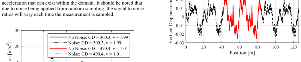
The central claim is that the variance of the front-axle vertical acceleration, together with vehicle speed, carries enough information to recover the road roughness parameter $GD$ (the scaled displacement power spectral density at 0.1 cycles/m) defined by ISO 8608, and that the recovery can be done online by Bayesian calibration. The BCR places a uniform prior on $GD$ over the interval 200 to 600, treats velocity as a known input in 0.5 to 2 m/s, and uses a Gaussian process surrogate trained on 198 Latin Hypercube samples of a simulated half-vehicle model to compute the likelihood. At run time, a moving buffer of the last 1000 acceleration samples at 120 Hz forms the observation, MCMC sampling with 5000 iterations and 1000 burn-in produces the posterior, and the posterior mean drives the controller. In simulated runs on a surface alternating between $GD$ 300 and 500, the BCR detects the transitions and the Simplex controller switches from performance mode to a fixed 1.0 m/s safety mode when the estimate exceeds 350.
Load-bearing premise
The real-time claim rests on the untested assumption that one MCMC calibration, with 5000 iterations and 1000 burn-in, finishes within the 8.33 seconds of data contained in the 1000-sample buffer at 120 Hz; the paper reports no computation time.
Editorial extensions
If this is right
- Roughness can be monitored continuously from IMU data alone, so no terrain map or prior knowledge of the route is required.
- The posterior distribution gives a quantitative confidence measure for each roughness estimate, which could be used to tune risk posture rather than relying on a single point value.
- With RMSE values of 42.6 and 94.4 for the $GD$ 300 and 500 segments without added noise, and 50.2 and 96.2 with noise, the current estimator is reliable enough to trigger mode switches but not to give fine-grained roughness values.
- The same calibration pipeline can be reused for another vehicle by retraining the surrogate on that vehicle's dynamic response, rather than redesigning the estimator.
- Accuracy degrades near the edges of the training domain, especially at low speed, so the operational envelope should stay away from those boundaries.
Reading between the lines
- The paper does not report the wall-clock time of one MCMC calibration; measuring it against the 8.33 s buffer window is the immediate test of whether the loop is truly real-time.
- Because the Simplex controller's safety mode is a fixed 1.0 m/s regardless of how far $GD$ exceeds the threshold, a natural extension would be a graded speed response that scales with roughness severity.
- The noise case only adds synthetic measurement noise; real suspension variability and model mismatch would likely require a larger training domain and more design points to keep the calibration accurate outside the B and C road classes.
- If the same approach moves to a physical vehicle, the half-vehicle surrogate would need to be validated against measured axle responses before the posterior can be trusted for control.
Editorial analysis
A structured set of objections, weighed in public.
Referee Report
Summary. The paper proposes a real-time road roughness estimation system for off-road autonomous vehicles. A Gaussian process surrogate is trained on 198 Latin Hypercube simulations of a half-vehicle model to map vehicle velocity and ISO 8608 road roughness (GD) to axle acceleration variance. A Bayesian calibration routine then inverts this mapping from observed acceleration variance and velocity to produce a posterior distribution for GD, using MCMC. The estimated GD feeds a Simplex controller that switches between a performance controller and a fixed 1.0 m/s safety mode. The system is tested in Isaac Sim on a 150 m terrain with GD=300 and GD=500 segments, under noiseless and noisy conditions, with three runs per case.
Significance. If the framework worked as described, it would be a useful demonstration of Bayesian calibration for terrain roughness estimation with quantified uncertainty in a control loop for small off-road robots. The approach is plausible in principle: using a GP surrogate is appropriate for expensive vehicle simulations, the post-predictive check is a good diagnostic, and running three stochastic repetitions is a reasonable attempt to show variability. However, the published control law is mathematically inconsistent with the reported experimental results, and the real-time computation premise is not verified by any timing data. These issues prevent assessing the actual significance of the claimed integrated system.
major comments (3)
- [Roughness based Simplex Control, Eq. (8)] The control law as written is self-contradictory. With GDmin=250 and GDmax=350, the performance-mode term Kp((GDmin+GDmax)/2 - GD(t)) equals Kp(300 - GD(t)). It is zero at GD=300 and strictly negative for 300<GD<=350 for every positive Kp. The test terrain's first and last 50 m have prescribed GD=300 (Fig. 8), so Eq. (8) commands v=0 on the nominal smooth segments and v=1.0 m/s only on the middle rough segment. Figures 10 and 12, which show positive cruise speeds and a reduction to a positive safety speed, cannot be outputs of this controller. The branch for GD<GDmin is also undefined, and no value of Kp is reported. This invalidates the integrated Simplex safety-modulation claim.
- [Bayesian Calibration Routine (BCR)] The real-time claim is load-bearing and unverified. The moving buffer is 1000 samples at 120 Hz, i.e., an 8.33 s window, and the active calibration performs 5000 MCMC iterations with 1000 burn-in plus additional step-size iterations. No computation time is reported. Without evidence that the posterior is produced within the buffer window, the abstract and conclusion's 'real-time' characterization is not established.
- [Assessment of the GPM-based Bayesian Calibration Method, Table 2] The operational domain is narrowed post hoc. Table 2 shows large calibration errors at v=0.75 m/s (e.g., 78.2% at GD=250, 33.6% at GD=300, 24.2% at GD=350), and the text then states that the routine 'doesn't behave as desired' for v<=0.75 m/s and excludes that range. The prior in Eq. (6) and the LHS training design, however, were defined over 0.5<=v<=2.0 m/s. The paper should either retrain and re-present the domain over v>0.75 m/s or justify the exclusion before claiming domain-wide performance; as written, the claim of real-time characterization across the stated velocity domain is unsupported.
minor comments (6)
- [Table 1] The row for Road Class B shows '32 28', which is likely a typo; ISO 8608 class B should extend from 32 to 128, and the table formatting is ambiguous.
- [Bayesian Calibration Routine (BCR)] The acronyms 'GPM', 'GP', and 'GPM/SA' are used interchangeably; an early explicit definition of all three would improve readability.
- [Calibration Metrics, Eq. (7)] The choice to normalize the variance by T rather than T-1 is stated but not justified; a brief explanation would help readers understand the calibration metric's statistical properties.
- [Figures 10 and 12] The vertical axis labels and the legend line indicating terrain roughness are not fully legible in the reproduction; please enlarge the fonts and line weights.
- [Bayesian Calibration Routine (BCR)] The text mentions that overlapping of buffer windows occurs because the buffer size is not directly related to travel length, but the overlap duration and its effect on mode-switching latency are not quantified; adding a sentence on this would be useful.
- [References] Reference [7] is an unpublished manuscript; providing a preprint or archival link would make the griddy Gibbs sampling approach verifiable.
Circularity Check
No circularity: the BCR is a genuine statistical inversion of an independently trained GP surrogate, and the self-citations are implementation/context rather than load-bearing.
full rationale
The paper's derivation chain is self-contained at the level of the simulation study. The BCR constructs a GP surrogate from 198 LHS-parameterized forward runs of the half-vehicle model (Section 'Simulations'), mapping (v, GD) to the scalar acceleration-variance metric f of Eq. 7, and then inverts this mapping through Bayes' rule (Eqs. 3-4) with stated uniform priors and MCMC. The posterior over GD is therefore a data-driven inverse estimate, not an input renamed as output; the metric f is not defined in terms of the calibrated GD, and the validation in Table 2 uses independently prescribed GD values rather than values fed back from the controller. The Simplex law in Eq. 8 is a control choice rather than a fitted parameter, and the reported speed reductions are not forced by construction of the BCR. Self-citations [7], [12], and [20] are used for code migration, related-work context, and road-profile generation; none supplies the central inferential result or a uniqueness/ansatz premise, so they are not load-bearing. The internal inconsistency of Eq. 8 (zero command at GD=300 and negative commands for 300<GD<=350) and the unreported MCMC latency are correctness/feasibility concerns, not circularity.
Assumptions & free parameters
free parameters (6)
- Proportional gain Kp =
not specified
- Control thresholds GDmin, GDmax =
250, 350
- MCMC run settings =
5000 iterations, 1000 burn-in; step size 1000/50
- Buffer size for acceleration variance =
1000 samples at 120 Hz
- Noise standard deviation sigma =
1
- Training domain bounds for GD and v =
GD in [200,600], v in [0.5,2] m/s
assumptions (5)
- standard math ISO 8608 GD value at 0.1 cycles/m quantifies road roughness
- domain assumption The GP surrogate accurately represents the Isaac Sim mapping f(v,GD) over the training domain
- domain assumption The road-profile generation reproduces the prescribed GD
- domain assumption The Clearpath Jackal in Isaac Sim can be approximated by a half-vehicle model with negligible damping and very high spring stiffness
- domain assumption Simplex architecture guarantees safe operation by switching to a fixed low speed when roughness exceeds threshold
Cite this review
Pith. "Pith review of Real-time Terrain Analysis for Off-road Autonomous Vehicles." pith.science (2026). https://pith.science/paper/MC2AQ4KL
@misc{pith2026250621347,
  author       = {Pith},
  title        = {Pith review of: Real-time Terrain Analysis for Off-road Autonomous Vehicles},
  year         = {2026},
  howpublished = {\url{https://pith.science/paper/MC2AQ4KL}},
  note         = {Machine review of arXiv:2506.21347}
}
read the original abstract
This research addresses critical autonomous vehicle control challenges arising from road roughness variation, which induces course deviations and potential loss of road contact during steering operations. We present a novel real-time road roughness estimation system employing Bayesian calibration methodology that processes axle accelerations to predict terrain roughness with quantifiable confidence measures. The technical framework integrates a Gaussian process surrogate model with a simulated half-vehicle model, systematically processing vehicle velocity and road surface roughness parameters to generate corresponding axle acceleration responses. The Bayesian calibration routine performs inverse estimation of road roughness from observed accelerations and velocities, yielding posterior distributions that quantify prediction uncertainty for adaptive risk management. Training data generation utilizes Latin Hypercube sampling across comprehensive velocity and roughness parameter spaces, while the calibrated model integrates seamlessly with a Simplex controller architecture to dynamically adjust velocity limits based on real-time roughness predictions. Experimental validation on stochastically generated surfaces featuring varying roughness regions demonstrates robust real-time characterization capabilities, with the integrated Simplex control strategy effectively enhancing autonomous vehicle operational safety through proactive surface condition response. This innovative Bayesian framework establishes a comprehensive foundation for mitigating roughness-related operational risks while simultaneously improving efficiency and safety margins in autonomous vehicle systems.
Figures


Figures from the paper (7 more)




Reference graph
Works this paper leans on
-
[1]
Z. Li, U. V . Kalabi ´c, I. V . Kolmanovsky, E. M. Atkins, J. Lu, and D. P. Filev, “Simultaneous road profile estimation and anomaly detection with an input observer and a jump diffusion process estimator,” in 2016 American Control Conference (ACC), pp. 1693–1698, 2016
work page 2016
-
[2]
The use of vehicle acceleration measurements to estimate road roughness,
Y .-Y . L. A. Gonz´alez, E.J. O’brien and K. Cashell, “The use of vehicle acceleration measurements to estimate road roughness,” Vehicle System Dynamics, vol. 46, no. 6, pp. 483–499, 2008
work page 2008
-
[3]
Estimation of road roughness condition from smartphones under realistic settings,
V . Douangphachanh and H. Oneyama, “Estimation of road roughness condition from smartphones under realistic settings,” in 2013 13th International Conference on ITS Telecommunications (ITST), pp. 433–439, 2013
work page 2013
-
[4]
A real time terrain recognition method for mobile robot moving,
J.-W. Chang, R.-J. Wang, and W.-J. Wang, “A real time terrain recognition method for mobile robot moving,” in 2016 International Conference on System Science and Engineering (ICSSE), pp. 1–4, 2016
work page 2016
-
[5]
These maps are made for walking: Real-time terrain property estimation for mobile robots,
P. Ewen, A. Li, Y . Chen, S. Hong, and R. Vasudevan, “These maps are made for walking: Real-time terrain property estimation for mobile robots,” IEEE Robotics and Automation Letters, vol. 7, no. 3, pp. 7083–7090, 2022
work page 2022
-
[6]
J. R. Gattiker, “Gaussian process models for simulation analysis (GPM/SA) command, function, and data structure reference,” tech. rep., Los Alamos National Laboratory
-
[7]
An efficent statistical inference approach for model calibration using griddy gibbs sampling
S. Wright, H. Stewart, S. Sharma, L. Redmond, C. Mcmahan, and M. Castanier, “An efficent statistical inference approach for model calibration using griddy gibbs sampling.” Unpublished Manuscript
-
[8]
Robot navigation in multi-terrain outdoor environments,
G. A. S. Pereira, L. C. A. Pimenta, A. R. Fonseca, L. de Q. Corrˆea, R. C. Mesquita, L. Chaimowicz, D. S. C. de Almeida, and M. F. M. Campos, “Robot navigation in multi-terrain outdoor environments,” The International Journal of Robotics Research, vol. 28, no. 6, pp. 685–700, 2009
work page 2009
Show all 24 references
-
[9]
Passivity-based model predictive control for mobile robot navigation planning in rough terrains,
A. Tahirovic and G. Magnani, “Passivity-based model predictive control for mobile robot navigation planning in rough terrains,” in 2010 IEEE/RSJ International Conference on Intelligent Robots and Systems, pp. 307–312, 2010
2010
-
[10]
Graspe: Graph based multimodal fusion for robot navigation in outdoor environments,
K. Weerakoon, A. J. Sathyamoorthy, J. Liang, T. Guan, U. Patel, and D. Manocha, “Graspe: Graph based multimodal fusion for robot navigation in outdoor environments,”IEEE Robotics and Automation Letters, vol. 8, pp. 8090–8097, Dec 2023
2023
-
[11]
A self-supervised terrain roughness estimator for off-road autonomous driving,
D. Stavens and S. Thrun, “A self-supervised terrain roughness estimator for off-road autonomous driving,” CoRR, vol. abs/1206.6872, 2012
2012 arXiv
-
[12]
Safety verification and navigation for autonomous vehicles based on signal temporal logic constraints,
A. Parameshwaran and Y . Wang, “Safety verification and navigation for autonomous vehicles based on signal temporal logic constraints,” tech. rep., SAE Technical Paper, 2023
2023
-
[13]
Safe and robust motion planning for dynamic robotics via control barrier functions,
A. Manjunath and Q. Nguyen, “Safe and robust motion planning for dynamic robotics via control barrier functions,” in 2021 60th IEEE Conference on Decision and Control (CDC), pp. 2122–2128, 2021
2021
-
[14]
R2-rrt*: Reliability-based robust mission planning of off-road autonomous ground vehicle under uncertain terrain environment,
C. Jiang, Z. Hu, Z. P. Mourelatos, D. Gorsich, P. Jayakumar, Y . Fu, and M. Majcher, “R2-rrt*: Reliability-based robust mission planning of off-road autonomous ground vehicle under uncertain terrain environment,” IEEE Transactions on Automation Science and Engineering, vol. 19...
2022
-
[15]
The simplex architecture for safe online control system upgrades,
D. Seto, B. Krogh, L. Sha, and A. Chutinan, “The simplex architecture for safe online control system upgrades,” in Proceedings of the 1998 American Control Conference. ACC (IEEE Cat. No. 98CH36207), vol. 6, pp. 3504–3508, IEEE, 1998
1998
-
[16]
Optimization of vehicle suspension parameters with use of evolutionary computation,
V . Goga and M. K ˇl´uˇcik, “Optimization of vehicle suspension parameters with use of evolutionary computation,” Procedia Engineering, vol. 48, p. 174–179, 12 2012
2012
-
[17]
Modelling of a mechanical system with one degree of freedom in matlab programme (in slovak),
P. Frankovsk ´y, I. Delyov´a, and D. Hroncov´a, “Modelling of a mechanical system with one degree of freedom in matlab programme (in slovak),” Transfer inov´aci´ı, pp. 71–73, 2011
2011
-
[18]
Model analysis of a mechanical system with two degrees of freedom in simulation environment matlab/simulink (in slovak),
I. Delyov ´a, D. Hroncov´a, and P. Frankovsk´y, “Model analysis of a mechanical system with two degrees of freedom in simulation environment matlab/simulink (in slovak),”ATP Journal plus, pp. 14–17, 2012
2012
-
[19]
ISO 8608:2016 mechanical vibration - road surface profiles - reporting of measured data,
International Organization for Standardization, “ISO 8608:2016 mechanical vibration - road surface profiles - reporting of measured data,” tech. rep., International Organization for Standardization, Switzerland, 2016
2016
-
[20]
Drive-by health monitoring of highway bridges using bayesian estimation technique for damage classification,
S. Mokalled, W. Locke, O. Abuodeh, L. Redmond, and C. McMahan, “Drive-by health monitoring of highway bridges using bayesian estimation technique for damage classification,” Structural Control and Health Monitoring, vol. 29, no. 6, p. e2944, 2022
2022
-
[21]
J. R. Gattiker and B. Williams, “Gpmsa.” https://github.com/lanl/GPMSA. Los Alamos Computer Code release LA-CC-06-079
-
[22]
Gelman, J
A. Gelman, J. B. Carlin, H. S. Stern, D. B. Dunson, A. Vehtari, and D. B. Rubin, Bayesian Data Analysis. CRC Press, third edition ed., 2013
2013
-
[23]
lhsdesign
MathWorks, “lhsdesign.” https: //www.mathworks.com/help/stats/lhsdesign.html. Accessed: September 20, 2024
2024
-
[24]
A comparison of three methods for selecting values of input variables in the analysis of output from a computer code,
M. D. McKay, R. J. Beckman, and W. J. Conover, “A comparison of three methods for selecting values of input variables in the analysis of output from a computer code,” Technometrics, vol. 21, no. 2, pp. 239–245, 1979. 8 Contact Information Edwina Lewis Graduate Research Assista...
1979
Reviewed August 6, 2026 · model on record in the stance chip above.
Discussion (0). Continue with ORCID to comment.