REVIEW 4 major objections 4 minor 1 cited by
Unfolding Generative Flows with Koopman Operators: Trajectory-Preserving Linearization
T0 review · 4 major / 4 minor · reviewed 2026-08-06 · deepseek-v4-flash
Pith's one-line read The paper claims that a single linear operator in a learned lifted space reproduces the full non-linear trajectory of a pre-trained flow-matching model, so sampling becomes one step and the operator's spectrum becomes a tool for…
desk verdict The consistency loss is a real step beyond endpoint distillation, but the paper's 'trajectory-preserving' claim currently rests on latent-space evidence; worth a serious review with a request for pixel-space trajectory metrics. read the letter →
The pith
A machine-rendered reading of the paper's core claim, the machinery that carries it, and where it could break.
The reading
What carries the argument
The central object is a learned finite-dimensional Koopman representation: a diffusion-style SongUNet encoder–decoder pair that maps the data space to a 1026-dimensional lifted space (1024 observables plus time and a constant coordinate), together with a dense affine generator matrix $L$ whose constrained block structure forces $\dot{t} = 1$ and $\dot{1} = 0$. The load-bearing identity is the Koopman generator equation $Lg = \nabla g \cdot v_t$, adapted from the autonomous-system generator formula to non-autonomous flow matching; the consistency loss is exactly the square of this equation averaged over the marginal path distribution. The mechanism that makes the objective trainable is the unbiased-estimator identity of Proposition 3, which rewrites the expectation over the unknown marginal path as an expectation over data samples and conditional paths — the simulation-free trick that makes CFM itself trainable, applied here with the teacher's known marginal velocity. Finally, the real Schur decomposition of $L$ splits the flow into independent exponential and spiral modes, and the paper orders these modes by their eigenvalues to reveal a coarse-to-fine hierarchy in generation.
What would settle it
Run the identical pipeline on a teacher whose dynamics are known to have no finite-dimensional Koopman invariant subspace — for instance a chaotic or polynomial flow of the kind discussed in the literature the paper cites on finite-dimensional Koopman forms — and record the consistency-loss residual and trajectory MSE at a large latent dimension. If the residual stays bounded well away from zero while endpoints still match, the trajectory-preserving claim is refuted: the method would be fitting boundaries and only approximating interiors. A complementary test that applies to the paper's own models is to compare intermediate marginals: integrate the teacher to a time $t \in (0,1)$ and compare the distribution of $x_t$ with one-step Koopman rollouts $\exp(tL)$ from the same noises; agreement at $t=1$ with divergence in the middle would falsify full-trajectory linearization.
Extended reading notes
Core claim
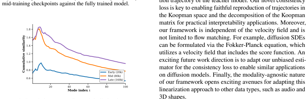
The central discovery, stated on the paper's own terms, is that a trajectory-preserving linearization of a pre-trained Conditional Flow Matching model exists and is learnable. For a teacher with velocity field $v_t$, the paper constructs an encoder $g_\phi$, a decoder $g_\psi^{-1}$, and a fixed generator matrix $L$ such that the lifted coordinate $z_t = [1, t, g_\phi(t, x_t)]$ evolves linearly, $\mathrm{d}z/\mathrm{d}t = Lz$, with the block structure of $L$ forcing time to advance at unit rate. The decisive ingredient is the consistency loss $L_{\mathrm{cons}} = \mathbb{E}\,\lVert L g(t,x_t) - \nabla g(t,x_t)\cdot v_t(x_t)\rVert^2$, which is an unbiased, simulation-free estimate of the true marginal objective (Proposition 3); the paper proves that the naive conditional substitute carries a positive gap (Proposition 2) and that the decoder's reconstruction loss fixes the coordinate freedom left by linear gauge invariance (Proposition 1). With this loss, one-step rollouts $x_1 \approx g^{-1}(\exp(L)z_0)$ reproduce teacher trajectories to mean squared error near $5\times10^{-6}$, whereas the same pipeline without the loss matches endpoints only, with error near $1.3\times10^{-3}$. The paper further reports that the spectrum of $L$ then carries meaning: Schur modes arrange coarse-to-fine, single-mode perturbations yield coherent attribute edits (sunglasses coherence 0.97), and images can be inverted back to noise through $\exp(-L)$.
Load-bearing premise
Everything rests on the assumption that the teacher's flow admits a finite-dimensional invariant Koopman subspace — that roughly 1024 learned coordinates are enough to make the teacher's dynamics exactly linear. The paper itself flags this as a strong condition that need not hold for arbitrary non-linear flows; if it fails, the consistency loss cannot approach zero and the linearization is only approximate.
Editorial extensions
If this is right
- Sampling from a CFM becomes one step — encode the noise, apply the matrix exponential once, decode — with the paper reporting FID 10.1 on FFHQ and 16.7 on CIFAR-10 at about 37 ms per image.
- The linearization is not a boundary fit: Koopman rollouts track the teacher's full trajectories to mean squared error near $5\times10^{-6}$ with the consistency loss, versus roughly $1.3\times10^{-3}$ without it.
- The spectrum of $L$ becomes a control surface: moving along a single Koopman mode edits attributes (CLIP coherence 0.97 for sunglasses, 0.94 for brown hair), and discovered directions transfer back into the original CFM's noise space.
- Inversion becomes a matrix exponential: $\exp(-L)$ sends images back to the teacher's noise space, which the paper uses for reconstruction and for downstream inpainting, super-resolution, and denoising.
- Because the consistency estimator needs only the teacher's velocity and marginals, the same linearization extends to any flow with an evaluable marginal velocity, including diffusion models via their probability-flow ODE.
Reading between the lines
- Editorial inference: if real-world flow models admit such faithful finite-dimensional Koopman representations, then editing, interpolation, and inversion of generative models reduce to linear algebra in one fixed basis — a learned Fourier analysis of generation — and the eigenvalue ordering itself becomes a compressed description of how a dataset's images are produced.
- Editorial inference: the consistency-loss residual is a measurable 'Koopman defect' per model, so it could be used as a diagnostic that ranks teachers or datasets by how far their dynamics are from linearizable; the paper builds this instrument but does not deploy it that way.
- Editorial inference: a direct testable extension is to run the same linearization inside the latent space of a high-resolution diffusion transformer, where the operator dimension stays near 1024 while image resolution grows; the paper's quality gap on harder datasets would then either close, supporting the invariant-subspace story, or persist, pointing to the encoder as the bottleneck.
- Editorial inference: the class-conditioned spectral signatures indicate that modes split into shared coarse structure and class-specific fine structure, suggesting a control scheme — steering class or identity by rescaling mode coefficients — that the paper does not itself propose.
Editorial analysis
A structured set of objections, weighed in public.
Referee Report
Summary. The paper proposes a Koopman-operator framework that linearizes the full generative dynamics of a pre-trained Continuous Flow Matching (CFM) model. The authors learn an encoder g_phi, a decoder g_psi^{-1}, and a linear generator matrix L such that the lifted coordinates evolve as dg/dt = L g, with an affine augmentation to handle the non-autonomous time dependence. The training objective combines phase, target, reconstruction, and a trajectory consistency loss; the consistency loss (Eq. 13) is claimed to be a simulation-free, unbiased estimator of the marginal consistency objective. Sampling is one-step via x1 = g^{-1}(exp(L) g(0, x0)). The paper further demonstrates applications in spectral mode analysis, semantic editing, inversion, and class-conditional spectral signatures, and reports competitive FID scores on MNIST, FFHQ, and CIFAR-10.
Significance. If the central trajectory-preservation claim is fully verified, this would be a meaningful advance: it would provide a single linear surrogate for the non-autonomous dynamics of a generative flow, enabling one-step parallel sampling while retaining fidelity to the teacher's intermediate states, and it would make spectral-analysis and control tools available for generative models. The paper is transparent about its main theoretical limitation (finite-dimensional invariant Koopman subspace), releases code, and includes an ablation clearly showing that the consistency loss is responsible for trajectory fidelity in the learned latent space. However, the current empirical verification is incomplete in a way that is load-bearing for the main claim: trajectory fidelity is only measured in the learned latent space, and the theoretical estimator is unbiased with respect to a mixture path rather than with respect to the teacher's actual ODE rollouts. The significance is therefore conditional on additional pixel-space trajectory evaluation.
major comments (4)
- [Sec. 6.2, Table 6] The trajectory-fidelity claim is supported only by latent-space comparisons: the authors encode teacher rollouts g(t, x_t) and compare them to exp(tL) g(0, x0) in the learned Koopman space. Because the reconstruction loss L_recon (Eq. 10) is applied only at t=1, no reported quantity constrains the decoder's output at intermediate times. A model could have small latent MSE while decoding to pixel-space states that do not match the teacher's intermediate images. Since the abstract and introduction explicitly claim full-trajectory preservation, the manuscript must report pixel-space trajectory fidelity, e.g., the MSE or LPIPS between g^{-1}(exp(tL)g(0,x0)) and the teacher ODE rollout x_t on shared noise seeds, at several times t (and with and without the consistency loss). Absent such a measurement, the central claim is not empirically established.
- [Sec. 4.3, Eq. (13)] Proposition 3 shows that Eq. (13) is an unbiased estimator of the marginal consistency loss with respect to the mixture path p_t(x) = ∫ p_t(x|x1) q(x1) dx1. However, the teacher's actual ODE trajectories are generated by the vector field v_t, and unless v_t is exactly the marginal velocity of p_t, the conditional-path samples are not distributed as teacher rollouts. For a pretrained CFM this holds only approximately, and it is precisely the approximation error that the linearization must tolerate. The paper should either justify that Eq. (13) controls the residual along true teacher rollouts, or quantify the discrepancy by evaluating the consistency residual on stored teacher trajectories and comparing it with the conditional-path estimate. Without this, 'trajectory-preserving' is only established relative to a surrogate path.
- [Sec. 6.3] The paper acknowledges that a finite-dimensional invariant Koopman subspace is 'a strong condition that need not hold for arbitrary nonlinear flows' and cannot be guaranteed a priori. This assumption is load-bearing: without it, the consistency loss cannot reach zero and the linearization is approximate. The current evidence (latent rollout MSE ~ 5e-6, competitive FID, and an intermediate optimal dimension in Fig. 5) is suggestive but indirect. A direct diagnostic would strengthen the claim significantly: report the held-out consistency-loss value L_cons (Eq. 13) and, ideally, the residual norm evaluated on actual teacher rollouts. If these residuals are not near zero, the paper should soften the trajectory-preservation claim accordingly.
- [Sec. 5.2 and Sec. 6.4, Table 2] The semantic-mode evaluation is partially circular: modes are selected using CLIP embedding similarity, and then coherence (Eq. 19) is measured with the same CLIP embeddings. This selection-evaluation loop inflates the reported coherence scores, especially for the 'with consistency' model. The interpretability claims should be validated with an independent attribute classifier or human evaluation, or the paper should explicitly state that the reported coherence is relative to the CLIP space used for discovery rather than an independent semantic measure.
minor comments (4)
- [Eq. (11)] The notation in Eq. (11) omits the time argument in the Jacobian: it should read ∇_x g_phi(t, x_t) · v_t(x_t), consistent with Eq. (13) and the surrounding text.
- [Fig. 3] The caption says 'N=400, 800, 100, full'; the third value is likely meant to be 1000 rather than 100.
- [Sec. 6.3 vs Fig. 5] The text states that 'the optimal FID value [is] at an intermediary Koopman dimension as seen in Figure 5', but the Figure 5 caption says 'the higher the dimension, the lower the FID'. These statements are inconsistent and should be reconciled.
- [Sec. 4.1, Eq. (7)] The block structure in Eq. (7) would be clearer if the dimensions of the blocks (b_g, A_gt, A_gg) were specified, since the augmented state mixes scalar time with vector-valued observables.
Circularity Check
CLIP-selected 'semantic modes' are scored by the same CLIP coherence metric, and latent-space trajectory fidelity is the training residual; the core Koopman linearization remains externally supervised by the teacher velocity field.
-
fitted input called prediction
[Section 5.2 (Eq. 19), Section 6.4 (Table 2), Appendix F.2, Appendix E.3]
"Binary attribute labels (e.g., smiling vs. not smiling, eyeglasses vs. no eyeglasses) are obtained via CLIP classification using natural-language prompts. ... these modes were not manually selected; rather, they were automatically identified by ranking all eigenmodes according to their CLIP coherence scores with respect to each attribute prompt. ... C^β_k = 1/N Σ_i sign(⟨CLIP(z'_k),CLIP(p_β)⟩−⟨CLIP(z),CLIP(p_β)⟩)"
Appendix F.2 discovers semantic directions from CLIP labels, and Appendix E.3 selects modes by ranking the Eq. 19 CLIP-coherence score. Table 2 then reports the maximum coherence for the same attributes and prompts. Because the mode-selection objective and the reported evaluation metric are the same CLIP embedding and the same attribute prompts, high coherence is partly guaranteed by the selection procedure; it is a restatement of the fitting criterion rather than independent evidence that the modes encode semantics.
-
fitted input called prediction
[Section 4.3 (Eq. 11 and 13), Section 6.2 (Table 1), Section 6.3]
"Lcons = E_{t, x_t∼p_t(x_t)} ||Lg_ϕ(t, x_t) − ∇_x g_ϕ(x_t)·v_t(x_t)||^2. ... We encode a teacher's trajectory {x_t}_{t∈[0,1]} in the latent space and compare this ground truth path z_t = g_ϕ(t, x_t) against the analytical linear trajectory from our model, z̃_t = exp(L̃t) z̃_0. We show the results in Table 1."
The reported trajectory MSE is an integrated version of the exact residual minimized by Lcons, evaluated in the same learned latent coordinates g. If the consistency residual is zero, then d/dt g(t,x_t) = Lg(t,x_t), so the rollout z̃_t = exp(tL)z_0 matches g(t,x_t) by construction; hence near-zero Table 1 MSE primarily reports convergence of the training objective. Section 6.3 then uses this same 'trajectory reproduction to within MSE ~10^-6' as evidence that a finite-dimensional Koopman representation exists, making that existence argument partly circular. Since L_recon is applied only at t=1, no independent image-space trajectory metric verifies intermediate-state preservation.
full rationale
The core linearization is not circular: Eq. 13 is a simulation-free estimator whose target is the pretrained teacher velocity field v_t, and Proposition 3's unbiasedness is a law-of-iterated-expectation identity, not a re-derivation of the teacher. The method is thus externally supervised rather than self-defined. No load-bearing self-citations appear. Two evaluation steps are partially circular, however. First, semantic modes are selected by ranking CLIP coherence (Eq. 19) and then reported as having high CLIP coherence for the same prompts, so the interpretability numbers in Table 2 are partly an artifact of selection. Second, 'trajectory fidelity' is measured in the learned latent space with a metric that is the integrated training residual Lcons; the paper's Section 6.3 even relies on this residual to argue that a finite-dimensional Koopman representation exists. The manuscript itself concedes in Sections 6.3 and 7 that finite-dimensional Koopman representability is not guaranteed a priori and that the quality gap widens on complex datasets, which is an honest limitation but does not remove the circularity of using the fitted residual as evidence. Overall, the central linearization claim retains independent content, but the interpretability and trajectory-preservation evidence are partially reduced to their own fitting criteria, yielding a score of 4.
Assumptions & free parameters
free parameters (5)
- Koopman latent dimension =
1026 (1024+2)
- Target loss weight with consistency =
0.01 (versus 1.0 without consistency)
- Edit strength alpha =
3.0 (Table 8)
- Number of pre-generated teacher pairs =
10^4 to 10^6 depending on dataset
- Unreported loss weights for phase and reconstruction terms =
not specified
assumptions (4)
- ad hoc to paper The Koopman generator L has a finite-dimensional invariant subspace of observables for the teacher CFM dynamics, and this subspace is learnable by the chosen encoder and decoder.
- domain assumption The teacher marginal vector field v_t is deterministic and can be evaluated at conditional samples x_t ~ p_t(·|x1).
- standard math Standard Koopman theory: composition of observables with the flow is linear, and the generator is the Lie derivative.
- standard math The augmented affine lift z = [1, t, g] with the block-structured generator in Eq. 7 enforces the time coordinate evolves as ?t = 1.
invented entities (1)
-
Koopman latent space and Koopman modes
Cite this review
Pith. "Pith review of Unfolding Generative Flows with Koopman Operators: Trajectory-Preserving Linearization." pith.science (2026). https://pith.science/paper/DJDGOQHX
@misc{pith2026250622304,
  author       = {Pith},
  title        = {Pith review of: Unfolding Generative Flows with Koopman Operators: Trajectory-Preserving Linearization},
  year         = {2026},
  howpublished = {\url{https://pith.science/paper/DJDGOQHX}},
  note         = {Machine review of arXiv:2506.22304}
}
read the original abstract
Continuous Normalizing Flows (CNFs) enable elegant generative modeling but remain bottlenecked by their iterative nature requiring costly sampling and lacking interpretability of the intermediate states. Recent approaches accelerate sampling by straightening trajectories or distilling endpoints, yet they treat the original generative process as a black box, discarding the teacher's intermediate dynamics. We propose a fundamentally different perspective: globally linearizing flow dynamics via Koopman theory to achieve trajectory-preserving linearization. By lifting a pre-trained Conditional Flow Matching (CFM) model into a higher-dimensional Koopman space, we represent its evolution with a single linear operator. Crucially, unlike boundary-only distillation, our method enforces infinitesimal consistency with the teacher's vector field along the full generative path. We derive a practical, simulation-free training objective that ensures this global alignment and yields two key benefits. First, sampling becomes one-step and parallelizable. Second, because the linearization is faithful to the dynamics, the Koopman operator provides unique insights on the generation. We demonstrate that this structure enables novel applications unavailable in prior approaches, including discovery of semantically coherent editing directions, inversion with a teacher-aligned linear operator and class-conditional spectral signatures. Empirically, our approach achieves competitive sample quality, while enabling spectral analysis and control of the entire trajectories of generative flows.
Figures


Figures from the paper (15 more)




Forward citations
Cited by 1 Pith paper
-
Koopman operator theory: fundamentals, control, and applications
Tutorial on Koopman operator theory, data-driven methods such as EDMD, and their use in controller design for nonlinear systems with provided simulations and code.
Reference graph
Works this paper leans on
-
[1]
Forecasting sequential data using consistent koopman autoencoders
Omri Azencot, N Benjamin Erichson, Vanessa Lin, and Michael Mahoney. Forecasting sequential data using consistent koopman autoencoders. In International Conference on Machine Learning, pages 475--485. PMLR, 2020
work page 2020
-
[2]
One-step offline distillation of diffusion-based models via koopman modeling
Nimrod Berman, Ilan Naiman, Moshe Eliasof, Hedi Zisling, and Omri Azencot. One-step offline distillation of diffusion-based models via koopman modeling. arXiv preprint arXiv:2505.13358, 2025
-
[3]
Koopman operator dynamical models: Learning, analysis and control
Petar Bevanda, Stefan Sosnowski, and Sandra Hirche. Koopman operator dynamical models: Learning, analysis and control. Annual Reviews in Control, 52: 0 197--212, 2021
work page 2021
-
[4]
Sam Bond-Taylor, Adam Leach, Yang Long, and Chris G Willcocks. Deep generative modelling: A comparative review of vaes, gans, normalizing flows, energy-based and autoregressive models. IEEE transactions on pattern analysis and machine intelligence, 44 0 (11): 0 7327--7347, 2021
work page 2021
-
[5]
Modern koopman theory for dynamical systems
Steven L Brunton, Marko Budi s i \'c , Eurika Kaiser, and J Nathan Kutz. Modern koopman theory for dynamical systems. arXiv preprint arXiv:2102.12086, 2021
arXiv 2021
-
[6]
Applied koopmanism
Marko Budi s i \'c , Ryan Mohr, and Igor Mezi \'c . Applied koopmanism. Chaos: An Interdisciplinary Journal of Nonlinear Science, 22 0 (4), 2012
2012
-
[7]
A survey on generative diffusion models
Hanqun Cao, Cheng Tan, Zhangyang Gao, Yilun Xu, Guangyong Chen, Pheng-Ann Heng, and Stan Z Li. A survey on generative diffusion models. IEEE Transactions on Knowledge and Data Engineering, 2024
2024
-
[8]
Neural ordinary differential equations
Ricky TQ Chen, Yulia Rubanova, Jesse Bettencourt, and David K Duvenaud. Neural ordinary differential equations. In Advances in Neural Information Processing Systems (NeurIPS), volume 31, 2018
work page 2018
Show all 49 references
-
[9]
Nice: Non-linear independent components estimation
Laurent Dinh, David Krueger, and Yoshua Bengio. Nice: Non-linear independent components estimation. In Workshop on Deep Learning, NIPS, 2014
2014
-
[10]
Density estimation using real nvp
Laurent Dinh, Jascha Sohl-Dickstein, and Samy Bengio. Density estimation using real nvp. In International Conference on Learning Representations (ICLR), 2017
2017
-
[11]
One step diffusion via shortcut models
Kevin Frans, Danijar Hafner, Sergey Levine, and Pieter Abbeel. One step diffusion via shortcut models. arXiv preprint arXiv:2410.12557, 2024
2024 arXiv
-
[12]
Koopman theory for generative modeling of chaotic time series
Margareta Grbi \'c , Qing Li, and Ioannis G Kevrekidis. Koopman theory for generative modeling of chaotic time series. Chaos: An Interdisciplinary Journal of Nonlinear Science, 31 0 (12), 2021
2021
-
[13]
Borgwardt, Malte J
Arthur Gretton, Karsten M. Borgwardt, Malte J. Rasch, Bernhard Sch \"o lkopf, and Alexander Smola. A kernel two-sample test. Journal of Machine Learning Research, 13 0 (25): 0 723--773, 2012. URL http://jmlr.org/papers/v13/gretton12a.html
2012
-
[14]
Gans trained by a two time-scale update rule converge to a local nash equilibrium, 2018
Martin Heusel, Hubert Ramsauer, Thomas Unterthiner, Bernhard Nessler, and Sepp Hochreiter. Gans trained by a two time-scale update rule converge to a local nash equilibrium, 2018. URL https://arxiv.org/abs/1706.08500
2018 arXiv
-
[15]
Denoising diffusion probabilistic models
Jonathan Ho, Ajay Jain, and Pieter Abbeel. Denoising diffusion probabilistic models. Advances in neural information processing systems, 33: 0 6840--6851, 2020
2020
-
[16]
Efficient 3d molecular generation with flow matching and scale optimal transport
Ross Irwin, Alessandro Tibo, Jon Paul Janet, and Simon Olsson. Efficient 3d molecular generation with flow matching and scale optimal transport. In ICML 2024 AI for Science Workshop, 2024
2024
-
[17]
Glow: Generative flow with invertible 1x1 convolutions
Diederik P Kingma and Prafulla Dhariwal. Glow: Generative flow with invertible 1x1 convolutions. In Advances in Neural Information Processing Systems (NeurIPS), volume 31, 2018
2018
-
[18]
u ske, P \'e ter Koltai, Hao Wu, Ioannis Kevrekidis, Christof Sch \
Stefan Klus, Feliks N \"u ske, P \'e ter Koltai, Hao Wu, Ioannis Kevrekidis, Christof Sch \"u tte, and Frank No \'e . Data-driven model reduction and transfer operator approximation. Journal of Nonlinear Science, 28: 0 985--1010, 2018
2018
-
[19]
Hamiltonian systems and transformation in hilbert space
Bernard O Koopman. Hamiltonian systems and transformation in hilbert space. Proceedings of the National Academy of Sciences, 17 0 (5): 0 315--318, 1931
1931
-
[20]
Dynamical systems of continuous spectra
Bernard O Koopman and John Von Neumann. Dynamical systems of continuous spectra. In Proceedings of the National Academy of Sciences, volume 18, pages 255--263. National Acad Sciences, 1932
1932
-
[21]
Dynamic mode decomposition: data-driven modeling of complex systems
J Nathan Kutz, Steven L Brunton, Bingni W Brunton, and Joshua L Proctor. Dynamic mode decomposition: data-driven modeling of complex systems. SIAM, 2016
2016
-
[22]
Flow matching for generative modeling
Yaron Lipman, Ioannis Gkioulekas, Tatsunori Hashimoto, William T Liu, Ben Poole, Ricky Richter-Powell, Robin Rombach, Ali Toker, and Jiaxin Wu. Flow matching for generative modeling. In International Conference on Learning Representations (ICLR), 2023
2023
-
[23]
Distilled decoding 1: One-step sampling of image auto-regressive models with flow matching
Enshu Liu, Xuefei Ning, Yu Wang, and Zinan Lin. Distilled decoding 1: One-step sampling of image auto-regressive models with flow matching. In The Thirteenth International Conference on Learning Representations, 2025
2025
-
[24]
Flow straight and fast: Learning to generate and transfer data with rectified flow, 2022
Xingchao Liu, Chengyue Gong, and Qiang Liu. Flow straight and fast: Learning to generate and transfer data with rectified flow, 2022. URL https://arxiv.org/abs/2209.03003
2022 arXiv
-
[25]
Flow straight and fast: Learning to generate straight lines improves generalization and efficiency
Xingchao Liu, Chengyue Gong, and Qiang Liu. Flow straight and fast: Learning to generate straight lines improves generalization and efficiency. In International Conference on Learning Representations (ICLR), 2023 a . Often referred to as Rectified Flow
2023
-
[26]
Flow matching with stochastic differential equations
Yujia Liu, Chuan Guo Li, Kuan-Chieh Zhou, and Anima Anandkumar. Flow matching with stochastic differential equations. arXiv preprint arXiv:2306.02393, 2023 b
2023
-
[27]
Latent consistency models: Synthesizing high-resolution images with few-step inference
Simian Luo, Yiqin Wu, Surui Wang, Puchao Chen, Shijie Zhao, Jun Zhu, et al. Latent consistency models: Synthesizing high-resolution images with few-step inference. arXiv preprint arXiv:2310.04378, 2023
2023 arXiv
-
[28]
Deep learning for universal linear embeddings of nonlinear dynamics
Bethany Lusch, J Nathan Kutz, and Steven L Brunton. Deep learning for universal linear embeddings of nonlinear dynamics. Nature communications, 9 0 (1): 0 4950, 2018
2018
-
[29]
Interpretable learning of effective dynamics for multiscale systems
Emmanuel Menier, Sebastian Kaltenbach, Mouadh Yagoubi, Marc Schoenauer, and Petros Koumoutsakos. Interpretable learning of effective dynamics for multiscale systems. In Proceedings A, volume 481, page 20240167. The Royal Society, 2025
2025
-
[30]
Spectral properties of dynamical systems, model reduction and decompositions
Igor Mezi \'c . Spectral properties of dynamical systems, model reduction and decompositions. Nonlinear Dynamics, 41: 0 309--325, 2005
2005
-
[31]
Koopman operator, geometry, and learning, 2020
Igor Mezic. Koopman operator, geometry, and learning, 2020. URL https://arxiv.org/abs/2010.05377
2020 arXiv
-
[32]
Linearly recurrent autoencoder networks for learning dynamics
Samuel E Otto and Clarence W Rowley. Linearly recurrent autoencoder networks for learning dynamics. SIAM Journal on Applied Dynamical Systems, 18 0 (1): 0 558--593, 2019
2019
-
[33]
Functional maps: a flexible representation of maps between shapes
Maks Ovsjanikov, Mirela Ben-Chen, Justin Solomon, Adrian Butscher, and Leonidas Guibas. Functional maps: a flexible representation of maps between shapes. ACM Transactions on Graphics (ToG), 31 0 (4): 0 1--11, 2012
2012
-
[34]
Pytorch: An imperative style, high-performance deep learning library, 2019
Adam Paszke, Sam Gross, Francisco Massa, Adam Lerer, James Bradbury, Gregory Chanan, Trevor Killeen, Zeming Lin, Natalia Gimelshein, Luca Antiga, Alban Desmaison, Andreas Köpf, Edward Yang, Zach DeVito, Martin Raison, Alykhan Tejani, Sasank Chilamkurthy, Benoit Steiner, Lu Fan...
2019 arXiv
-
[35]
Pedregosa, G
F. Pedregosa, G. Varoquaux, A. Gramfort, V. Michel, B. Thirion, O. Grisel, M. Blondel, P. Prettenhofer, R. Weiss, V. Dubourg, J. Vanderplas, A. Passos, D. Cournapeau, M. Brucher, M. Perrot, and E. Duchesnay. Scikit-learn: Machine learning in P ython. Journal of Machine Learnin...
2011
-
[36]
State of the art on diffusion models for visual computing
Ryan Po, Wang Yifan, Vladislav Golyanik, Kfir Aberman, Jonathan T Barron, Amit Bermano, Eric Chan, Tali Dekel, Aleksander Holynski, Angjoo Kanazawa, et al. State of the art on diffusion models for visual computing. In Computer Graphics Forum, volume 43, page e15063. Wiley Onli...
2024
-
[37]
Multisample flow matching: Straightening flows with minibatch couplings
Aram-Alexandre Pooladian, Alexander Gushchin, Regina Barzilay, and Tommi Jaakkola. Multisample flow matching: Straightening flows with minibatch couplings. arXiv preprint arXiv:2305.17160, 2023
2023 arXiv
-
[38]
U-net: Convolutional networks for biomedical image segmentation, 2015
Olaf Ronneberger, Philipp Fischer, and Thomas Brox. U-net: Convolutional networks for biomedical image segmentation, 2015. URL https://arxiv.org/abs/1505.04597
2015 arXiv
-
[39]
Spectral analysis of nonlinear flows
Clarence W Rowley, Igor Mezi \'c , Shervin Bagheri, Philipp Schlatter, and Dan S Henningson. Spectral analysis of nonlinear flows. Journal of fluid mechanics, 641: 0 115--127, 2009
2009
-
[40]
Generative modeling by estimating gradients of the data distribution
Yang Song and Stefano Ermon. Generative modeling by estimating gradients of the data distribution. Advances in neural information processing systems, 32, 2019
2019
-
[41]
Score-based generative modeling through stochastic differential equations
Yang Song, Jascha Sohl-Dickstein, Diederik P Kingma, Abhishek Kumar, Stefano Ermon, and Ben Poole. Score-based generative modeling through stochastic differential equations. arXiv preprint arXiv:2011.13456, 2020
2011 arXiv
-
[42]
Consistency models
Yang Song, Prafulla Dhariwal, Mark Zhang, and Karsten Kreis. Consistency models. In International Conference on Machine Learning (ICML), 2023
2023
-
[43]
Strogatz
Steven H. Strogatz. Nonlinear Dynamics and Chaos: With Applications to Physics, Biology, Chemistry and Engineering. Westview Press, 2000
2000
-
[44]
Applied koopman operator theory for power systems technology
Yoshihiko Susuki and Igor Mezi \'c . Applied koopman operator theory for power systems technology. Nonlinear theory and its applications, IEICE, 7 0 (4): 0 430--459, 2016
2016
-
[45]
Conditional flow matching: Simulation-free dynamic optimal transport
Alexander Tong, Nikolay Malkin, Guillaume Huguet, Yanlei Zhang, Jarrid Liu, Kilian Rector-Brooks, Guy Wolf Fatras, Elizabeth Creager, and Yoshua Bengio. Conditional flow matching: Simulation-free dynamic optimal transport. arXiv preprint arXiv:2302.00482, 2023 a
2023 arXiv
-
[46]
Improving and generalizing flow-based generative models with minibatch optimal transport
Alexander Tong, Kilian FATRAS, Nikolay Malkin, Guillaume Huguet, Yanlei Zhang, Jarrid Rector-Brooks, Guy Wolf, and Yoshua Bengio. Improving and generalizing flow-based generative models with minibatch optimal transport. Transactions on Machine Learning Research, 2024. ISSN 283...
2024
-
[47]
Torchcfm: A conditional flow matching library
Alexander Tong et al. Torchcfm: A conditional flow matching library. https://github.com/atong01/conditional-flow-matching, 2023 b
2023
-
[48]
Diffusion models: A comprehensive survey of methods and applications
Ling Yang, Zhilong Zhang, Yang Song, Shenda Hong, Runsheng Xu, Yue Zhao, Wentao Zhang, Bin Cui, and Ming-Hsuan Yang. Diffusion models: A comprehensive survey of methods and applications. ACM Computing Surveys, 56 0 (4): 0 1--39, 2023
2023
-
[49]
Learning deep neural network representations for koopman operators of nonlinear dynamical systems
Enoch Yeung, Soumya Kundu, and Nathan Hodas. Learning deep neural network representations for koopman operators of nonlinear dynamical systems. In 2019 American Control Conference (ACC), pages 4832--4839. IEEE, 2019
2019
Reviewed August 6, 2026 · model on record in the stance chip above.
Discussion (0). Sign in to comment.