Solving inverse problems of Type IIB flux vacua with conditional generative models

Sven Krippendorf; Zhimei Liu

REVIEW 4 major objections 4 minor 1 cited by

Solving inverse problems of Type IIB flux vacua with conditional generative models

T0 review · 4 major / 4 minor · reviewed 2026-08-06 · deepseek-v4-flash

Challenge this review Re-run · record.json Download PDF Read on arXiv ↗

Pith's one-line read A conditional variational autoencoder can generate new, physically valid Type IIB flux vacua with a chosen superpotential about a thousand times faster than Metropolis sampling.

desk verdict Useful proof-of-concept for CVAE-based flux generation, but the 'beyond training set' claim is unverified and the finite-box support limits the inverse-problem framing. read the letter →

arxiv 2506.22551 v1 pith:ATISNGER submitted 2025-06-27 hep-th hep-ph

Sven Krippendorf , Zhimei Liu This is my paper

classification hep-thhep-ph

keywords TypeIIBfluxcompactificationsvacuainverseproblemconditionalvariationalautoencodersuperpotentialstringlandscapeMetropolissamplingtadpoleconstraint

verification ladder T0 review T1 audit T2 compute T3 formal

The pith

A machine-rendered reading of the paper's core claim, the machinery that carries it, and where it could break.

The reading

This paper argues that the inverse problem of Type IIB flux compactifications—finding integer flux vectors $x$ that yield vacua with a specified low-energy property, here a target value of the superpotential $|W_0|$—can be solved by a conditional variational autoencoder (CVAE). The model is trained on several thousand to tens of thousands of physically valid flux vectors, conditioned on $|W_0|$ ranges, and augmented with loss terms that encode the D3-brane tadpole charge $N_{flux}$ and the superpotential. On a conifold and a symmetric torus, generated samples reproduce the joint $(N_{flux}, |W_0|)$ distribution and the marginal statistics of the flux numbers, reach narrow target windows at rates that degrade gracefully as the window shrinks, and include many distinct vectors absent from the training data. The paper reports a sampling speedup of about $O(10^3)$ relative to a Metropolis baseline in narrow $|W_0|$ windows, with the speedup growing as the window narrows. If correct, this gives a scalable way to probe finely tuned corners of the string landscape and to estimate conditional distributions over flux vacua.

What carries the argument

The central object is a Conditional Variational Autoencoder (CVAE): a variational autoencoder whose decoder receives a latent code concatenated with a condition label $c$, so that samples can be drawn for a chosen class. For flux vacua, $x$ is one-hot encoded component-wise, so a vector in $[-30,30]^8$ becomes a 488-dimensional input; the encoder maps this to a factorized Gaussian latent distribution, and a linear classifier on the latent mean encourages labels to cluster. The training objective is a weighted sum of reconstruction loss, KL divergence, classification loss, and two physics losses—mean squared error on $N_{flux}$ and mean absolute error on $|W_0|$—so the decoder learns to avoid unphysical flux vectors even before post-selection. At generation time, the decoder is fed a latent vector sampled from class-conditional latent statistics (or from the standard normal prior for continuous labels) together with the desired label; the output is decoded to integer flux components and post-selected with the physical constraints. The class-conditioned latent structure plus the physics-informed losses are what let the model propose valid, targeted configurations without solving the F-term equations during sampling.

What would settle it

An end-to-end experiment on an enlarged box would settle the claim: build training data in $[-60,60]^8$ on the conifold, train the CVAE, and compare the total wall-clock time—including dataset construction, the roughly 300 training epochs, and sampling—needed to produce a fixed number of valid samples in a narrow $|W_0|$ window against the Metropolis baseline. If the CVAE is not faster from scratch, or if it never proposes valid vacua whose flux components lie outside $[-30,30]^8$, then the method's coverage and speedup are limited to the preselected box and post-training sampling.

Watch

Extended reading notes

Core claim

The paper's central claim is that a CVAE whose loss contains physical constraints can learn the conditional distribution $P(x | N_{flux}, |W_0|)$ over integer flux vectors satisfying the F-term conditions, the tadpole bound, and the dilaton fundamental-domain gauge fixing, and can sample from it far more cheaply than a random-walk Metropolis chain. On the conifold with $L_{max}=972$ and target $|W_0|=40,000±500$, 100,000 generated samples yield on average 13,209 physically valid vectors, 5,975 of them distinct, from a training class containing 992 vectors; in every one of the five target windows the distinct generated count exceeds the training count. On the symmetric torus with $L_{max}=500$, the same procedure finds a smallest $|W_0|=0.007294$, consistent with earlier searches that reached about $10^{-2}$, and the smallest values occur at large $N_{flux}$. The paper frames itself as a method paper: the point is the machinery for targeted generation and the $O(10^3)$ speedup, not a claim about the global distribution of vacua.

Load-bearing premise

The method assumes that the physically interesting flux vectors lie inside the fixed integer range used to construct the training set (on the conifold $[-30,30]^8$, on the torus $[-3,3]^8$ or $[-20,20]^8$), because the model cannot represent integers outside that range.

Editorial extensions

If this is right

Within the training box, a single model with continuous labelling can target any $|W_0|$ value in the learned range without retraining, whereas genetic-algorithm searches must be rerun with new parameters for each target range.
The number of distinct valid flux vectors generated in each target window exceeds the number of training vectors in that window, so the model is proposing genuinely new configurations, not recalling memorised training points.
The sampling speedup grows as the target window narrows, so the method becomes more advantageous exactly where rejection sampling and MCMC are slowest.
By construction, the trained model makes conditional distributions such as $P(x | N_{flux}, |W_0|)$ accessible, which the paper argues is useful for comparing how common or rare particular vacuum properties are in the sampled region.
On the symmetric torus, the small-$|W_0|$ values found by the CVAE sit at large $N_{flux}$, matching the paper's expectation that discrete-flux effects obscure $W_0=0$ at small $L_{max}$.

Reading between the lines

Editorial extensions of the paper, not claims the author makes directly.

Inference: the reported $O(10^3)$ speedup measures post-training sample generation. An end-to-end comparison that includes the roughly 300 training epochs and the cost of building the training set by random sampling would give a fairer picture of when the CVAE beats Metropolis on total wall-clock time.
Inference: because the one-hot encoding restricts all outputs to the training box, the method's coverage of the landscape is bounded by that box. A direct test would train on an enlarged box and check whether target-region accuracy and the speedup survive; the paper gives no evidence that all physically interesting vacua lie inside $[-30,30]^8$ or $[-20,20]^8$.
Inference: the same conditioning structure could be applied to other targets—string coupling $g_s$, complex-structure masses, or $N_{flux}$ itself—and, if latent clustering persists in higher-dimensional flux spaces, would provide conditional vacuum statistics that Metropolis cannot reach in reasonable time.
Inference: the claim that generated configurations are novel is based on distinct flux vectors; a stricter check would compare derived physical quantities such as moduli VEVs, mass spectra, and axio-dilaton values between generated and training vacua, since different integer vectors can still approximate the same vacuum.

Share X Bluesky LinkedIn Reddit HN

Editorial analysis

A structured set of objections, weighed in public.

Desk editor's note, referee report, and a circularity audit.

Desk Editor's Note

read the letter

Good paper to know about, but read the claims carefully. The core result is a conditional VAE that, after training on discrete Type IIB flux vectors filtered by physical constraints, can generate new flux vectors in a targeted |W0| window with much lower sampling cost than a Metropolis baseline. That is genuinely new for this application: prior ML work used genetic algorithms or RL, and the generative-model papers didn't condition on physical targets over discrete flux space. The two geometries, conifold and symmetric torus, are small but nontrivial, and the authors do a decent job comparing marginal distributions and correlations of the generated samples against training data and Metropolis output.

The soft spots are real but not fatal. The biggest is the 'beyond the training set' claim. The count of distinct generated vectors exceeding the count of training vectors does not establish novelty; without an overlap check, most of those distinct vectors could be in the training set. The paper never checks whether generated vectors actually avoid the training set. That should be easy to do and would settle the claim.

The second issue is the decoder's support. One-hot encoding restricts every component to the box used for training ([-30,30] for the conifold), so the model can only propose fluxes inside that box. The tadpole bound is bilinear and does not force components into such a box, so the paper is solving the inverse problem over a preselected subset, not the full flux lattice. The Metropolis baseline shares the same box, so the speedup comparison is internally fair, but the external-validity gap is unquantified. The paper never says how many physically valid vacua lie outside the box.

Third, the O(10^3) speedup counts only post-training sampling. Training takes time and compute, and the paper doesn't report training cost. That's a minor omission for a proof of concept, but the abstract's phrasing is stronger than the evidence.

The absence of code and data is a practical inconvenience; the method is reproducible in principle but would be easier to evaluate with the artifacts.

Overall, this is a solid proof of concept that deserves a serious referee. A referee should ask for the overlap check, an explicit statement about the box limitation, and training-time reporting. I'd send it to review.

Referee Report

4 major / 4 minor

Summary. The paper proposes a conditional variational autoencoder (CVAE) framework for the inverse problem of Type IIB flux compactifications: given a target superpotential magnitude |W0| (or a range), generate discrete integer flux vectors that satisfy the physical vacuum conditions. The model is trained on datasets of flux vectors that already pass physical constraints, using a loss function that combines reconstruction, KL divergence, a classification or regression term on the label, and auxiliary physics losses on Nflux and |W0|. The authors test the method on two one-modulus geometries, a conifold in WP^4_{1,1,1,1,4} and the symmetric torus T^6, and compare against a Metropolis baseline. They report that the CVAE reproduces the training-set marginals and correlations, achieves an O(10^3) sampling speedup over Metropolis in narrow |W0| ranges, and generates more distinct flux vectors than are present in the training set, which they interpret as evidence of generalization beyond the training data. The paper is framed explicitly as a proof-of-concept method paper.

Significance. If the claims are fully supported, the paper would be a useful proof of concept: it demonstrates a generative-model pipeline that can propose discrete flux vectors conditioned on a physical target, which is a genuinely different approach from continuous-flux statistical methods and from genetic-algorithm or reinforcement-learning searches. The explicit use of physics-informed loss terms and the comparison to a Metropolis baseline are appropriate steps for a methods paper. The main strengths are the clear statement of the sampling task, the two concrete test geometries with explicit flux and tadpole formulas, and the reproducible experimental setup described in the appendices. However, the significance is currently limited by three gaps: the 'novel beyond training data' claim is not actually tested, the speedup figure excludes training cost, and the entire method is restricted to a preselected finite integer box whose coverage of physically relevant vacua is not established. These gaps do not destroy the core proof-of-concept, but they do require the central claims to be substantially qualified and, in part, re-verified before the paper can be accepted.

major comments (4)

[§4.1.1, Tables 1 and 2] The claim that the number of distinct generated flux vectors exceeding the number of training data indicates novelty 'beyond the training dataset' is not supported by the statistics presented. The fourth and fifth columns of Tables 1 and 2 count generated vectors and distinct generated vectors among the 100,000 samples, respectively; they do not measure the overlap between generated samples and the training set. A model that mostly reproduces training vectors would also show many distinct generated vectors if the generation count is large. To support the abstract and Section 5 claims, the authors should report, for each experiment, how many generated distinct vectors are absent from the training set (e.g., by exact set subtraction or by checking equality with training vectors), and how many training vectors are never generated.
[Appendix B, §4.1.1, §4.2.1, Appendix A] The inverse problem is solved only over a finite integer box. The one-hot encoding in Appendix B restricts every generated component to [-30,30] for the conifold, and Section 4.2.1 uses [-3,3]^8 or [-20,20]^8 for the torus; the Metropolis baseline is likewise restricted to the same box in Appendix A, Step 3. The tadpole constraint 0 < Nflux < Lmax is bilinear in the flux vector and does not imply a componentwise bound, so there is no a priori reason that all physically interesting vacua lie inside the chosen box. The paper does not quantify how many vacua in the target |W0| ranges fall outside the box or how sensitive the results are to the box choice. The authors should either provide such coverage statistics or explicitly reframe the central claim as solving the inverse problem over a preselected finite box, not over the full flux lattice.
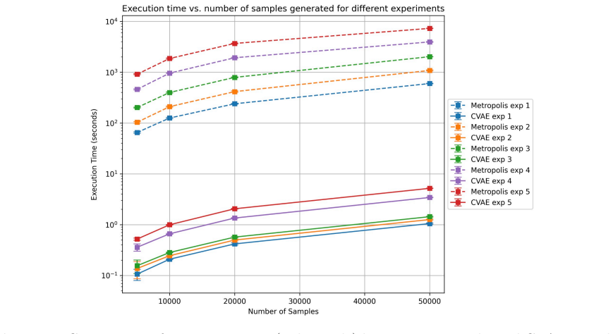
[§4.1.2, Figure 5] The reported O(10^3) speedup compares only post-training sampling times. The total cost of the method includes roughly two hours of dataset generation on a MacBook Air M1 (Section 4.1.1) plus model training to epoch 300 (Appendix B), and the Metropolis baseline requires no training phase. The amortized speedup may still be large when many samples or many target ranges are needed, and the continuous-label experiment in Section 4.3 is a good illustration of that amortization, but the paper should state the training time explicitly and qualify the speedup claim as a sampling-time speedup rather than an end-to-end speedup for a single target.
[§3.1, Tables 1 and 2, Appendix A] The physical-validity comparison is not fully transparent because the CVAE pipeline includes post-selection. The text states in Section 3.1 that generated samples are post-selected to satisfy constraints (2.6), (2.8), and (2.10), and the fourth column of Tables 1 and 2 counts only physically valid vectors. The Metropolis baseline, by construction, returns only accepted states. The paper should report the raw generation acceptance rate (before post-selection) for the CVAE, and should clarify that the Metropolis-CVAE comparison is between a sampler with built-in validity and a generative model followed by filtering. This does not invalidate the comparison, but it is necessary for a fair interpretation of both the speedup and the 'physical consistency' of the generated samples.

minor comments (4)

[Throughout] There are several typographical issues, for example 'T able 1' on page 10, 'CV AEs' with inconsistent spacing in the abstract and introduction, and an extra space in 'WP4 1,1,1,1,4' in a few places. A careful proofread is recommended.
[§4.2.1, Table 2] The class structure for Experiments 2 through 5 is not specified precisely. The text says 'more classes are being divided' but does not provide the label boundaries for each experiment. Please list the class thresholds or refer to the dataset construction details.
[Figure 5] The vertical axis is labeled in log scale but the tick labels and units are not fully described; please specify whether the times are in seconds and whether the error bars are standard deviations over the five runs mentioned in the caption.
[§4.3, Figure 11] The residual plot is described but not shown in the text; please ensure the figure actually includes the residual panel, or adjust the description.

Circularity Check

0 steps flagged · score 0.0 of 10

No significant circularity; the CVAE generation is benchmarked against first-principles physical constraints and an independent Metropolis runtime comparison.

full rationale

The paper's central claims are (i) that a CVAE can generate physically valid flux vectors conditioned on a target |W0| range, (ii) that this is faster than Metropolis sampling, and (iii) that many generated vectors are distinct from the training set. None of these claims reduces by construction to the training data or to a fitted parameter. The conditional label c is an input to the decoder, not a quantity re-derived from the output; whether the decoder maps c to vectors whose physical |W0| lies in the requested bin is an empirical question, and the physical validity of a generated vector is checked against the independent F-term and tadpole conditions (2.6), (2.8), and (2.10). The Metropolis baseline is fitted to a KDE of the same training set, so the agreement of marginal distributions and correlations with the training set is largely a self-consistency check rather than an external validation, but the speedup comparison is an external runtime benchmark against an independent sampling algorithm, and the novelty claim is evaluated by set difference from the training data plus first-principles constraints. The paper's self-citations [16,17,23,24,25] are used for conventions, empirical motivation, numerical tools, and cross-checks with earlier RL/GA results; none carries the central derivation, no uniqueness theorem is imported from the authors' prior work, and no ansatz is smuggled in via citation. The restriction of all flux components to finite boxes is a genuine external-validity limitation, but it is a modeling assumption, not a circular step. Overall, the derivation chain is self-contained and the central claims have independent content.

Assumptions & free parameters 4 free parameters · 4 assumptions · 0 invented entities

The central claim rests on the standard Type IIB flux vacuum formalism, a near-conifold period approximation, and the choice of a finite training box. The fitted quantities are ML hyperparameters and the box ranges; no new physical entities are introduced.

free parameters (4)

Flux box bounds for training set = [-30,30]^8 (conifold), [-3,3]^8 and [-20,20]^8 (torus)
Chosen by hand; the one-hot encoding restricts every generated flux component to this box, so it defines the search space for the inverse problem.
Loss weights alpha1, alpha2, alpha3, alpha4 = 0.1, 100, 50, 0.1
Set after hyperparameter search in Appendix B; they control the balance between reconstruction, KL, classification, and physical losses, and affect generation accuracy.
Latent dimension and hidden layer sizes = latent 32; hidden 512, 256, 128
Chosen by hyperparameter search; no ablation is reported, so the dependence of the results on these values is unknown.
Metropolis KDE bandwidth and proposal step size gamma = not reported numerically
The KDE bandwidth is grid-searched and gamma is described as tunable in Appendix A; these choices influence the baseline runtime and therefore the claimed speedup.

assumptions (4)

domain assumption The F-term conditions (2.6), tadpole bound (2.8), and fundamental domain (2.10) correctly define the set of physical flux vacua.
Inherited from the Type IIB flux literature; these conditions are used to filter both the training data and the generated samples.
domain assumption The near-conifold period expansions (4.2) and the derived formula for ln(x) in (4.3) are accurate over the sampled flux range.
The formulas are taken from [40], but the paper gives no error estimate, and the same approximation is used to validate generated vacua.
ad hoc to paper Random sampling inside the chosen integer box followed by physical filtering yields a representative sample of the conditional vacuum distribution.
The learned distribution inherits the box and the sampling proposal; no reweighting, coverage check, or comparison to an independent sample is provided.
ad hoc to paper The kernel density estimate of the training set is a good target distribution for the Metropolis baseline.
Appendix A builds the Metropolis acceptance rule on this KDE; if the KDE is inaccurate, the baseline is slower or biased and the speedup comparison is distorted.

how reviews work

0 comments

Cite this review

Pith. "Pith review of Solving inverse problems of Type IIB flux vacua with conditional generative models." pith.science (2026). https://pith.science/paper/ATISNGER

@misc{pith2026250622551,
  author       = {Pith},
  title        = {Pith review of: Solving inverse problems of Type IIB flux vacua with conditional generative models},
  year         = {2026},
  howpublished = {\url{https://pith.science/paper/ATISNGER}},
  note         = {Machine review of arXiv:2506.22551}
}

abstract

We address the inverse problem in Type IIB flux compactifications of identifying flux vacua with targeted phenomenological properties such as specific superpotential values or tadpole constraints using conditional generative models. These machine learning techniques overcome computational bottlenecks in traditional approaches such as rejection sampling and Markov Chain Monte Carlo (MCMC), which struggle to generate rare, finely-tuned vacua. As a proof of concept, we demonstrate that conditional generative models provide a more efficient alternative, specifically using conditional variational autoencoders (CVAEs). We introduce a CVAE framework tailored to flux compactifications, incorporating physical constraints directly into the loss function - enabling the generation of physically consistent vacua beyond the training set. Our experiments on conifold and symmetric torus background geometries show that the CVAE achieves a speedup of about $O(10^3)$ compared to Metropolis sampling, particularly in narrow target ranges for superpotential values. Additionally, the CVAE generates novel, distinct flux configurations beyond the training data, highlighting its potential for probing computationally challenging regions of the string landscape. Our results establish conditional generative models as a powerful and scalable tool for targeted flux vacua generation, opening new pathways for model building in regions of the landscape previously inaccessible by traditional model building techniques.

Figures

Figures reproduced from arXiv: 2506.22551 by the authors.

**Figure 1.** Schematic overview of our Conditional Variational Autoencoder (CVAE) architecture. The encoder maps the input flux vector x ∈ Z 8 to a latent distribution qϕ(z|x), parameterized by the mean µ and log-variance log σ 2 . A latent sample z is drawn from this distribution and concatenated with the condition label c before being passed to the decoder. The decoder reconstructs the input from pθ(x|z, c). loss, which outp… view at source ↗

**Figure 2.** Comparison of the distributions of Nflux and |W0| between the training set (left) and the CVAE-generated samples (right) for the conifold, targeting the region |W0| = 40,000±10,000 (Experiment 1 in [PITH_FULL_IMAGE:figures/full_fig_p011_2.png] view at source ↗

**Figure 3.** Comparison of marginal distributions for each flux number between the training set, Metropolis-generated samples and CVAE-generated samples, targeting |W0| = 40,000±500 (Experiment 5 in [PITH_FULL_IMAGE:figures/full_fig_p012_3.png] view at source ↗

Figures from the paper (11 more)

**Figure 4.** Figure 4: Conifold: Correlation heatmaps of flux numbers for the training set, Metropolisgenerated samples and CVAE-generated samples, targeting |W0| = 40,000 ± 500 (Experiment 5 in [PITH_FULL_IMAGE:figures/full_fig_p013_4.png]

**Figure 5.** Figure 5: Comparison of execution times (in log scale) between Metropolis and CVAE sampling methods on the conifold, with 5,000, 10,000, 20,000 and 50,000 samples generated in each of the five experiments. Error bars indicate standard deviations computed over five independent ru…

**Figure 6.** Figure 6: Comparison of the distributions of Nflux and |W0| between the training set (left) and the CVAE-generated samples (right) for the symmetric torus, targeting the region |W0| < 20 (Experiment 1 in [PITH_FULL_IMAGE:figures/full_fig_p016_6.png]

**Figure 7.** Figure 7: Comparison of marginal distributions for each flux number between the training set, Metropolis-generated samples and CVAE-generated samples, targeting |W0| < 20 (Experiment 1 in [PITH_FULL_IMAGE:figures/full_fig_p017_7.png]

**Figure 8.** Figure 8: Correlation heatmaps of flux numbers for the training set, Metropolis-generated samples and CVAE-generated samples, targeting |W0| < 20 (Experiment 1 in [PITH_FULL_IMAGE:figures/full_fig_p018_8.png]

**Figure 9.** Figure 9: Distribution of |W0| < 0.3 vacua in dilaton fundamental domain (top) and in complex structure fundamental domain (bottom) for Lmax = 500 for the training set and CVAE-generated samples. 18 [PITH_FULL_IMAGE:figures/full_fig_p019_9.png]

**Figure 10.** Figure 10: Scatter plot between |W0| and Nflux for CVAE-generated flux vectors with continuous labeling on the conifold. The target |W0| values are 20,000, 40,000, 60,000, 80,000 and 100,000, each with 2,000 generated samples (which takes about 0.1 seconds on a MacBook Air M1 t…

**Figure 11.** Figure 11: Linear regression between the target and predicted |W0| values for CVAE-generated flux vectors. The line of best fit is |Wˆ 0| = 0.931 |W0| + 4012.80. The residuals, shown in the lower panel, cluster around zero, indicating no systematic bias. confirms this, showing t…

**Figure 12.** Figure 12: Top: Comparison of the marginal distributions for Nflux (left) and |W0| (right) between the training set and Metropolis-generated samples on the conifold, targeting |W0| = 40,000 ± 500. A total of 2,000 samples were generated using Metropolis. Bottom: Comparison of th…

**Figure 13.** Figure 13: Loss curves for Experiment 1 in [PITH_FULL_IMAGE:figures/full_fig_p025_13.png]

**Figure 14.** Figure 14: Left: average prediction accuracy curve during training. Right: latent space visualization using t-SNE for Experiment 1 in [PITH_FULL_IMAGE:figures/full_fig_p025_14.png]

Discussion (0). Sign in to comment.

Forward citations

Cited by 1 Pith paper

Reviewed papers in the Pith corpus that reference this work. Sorted by Pith novelty score. Full citation record

When minor issues matter: symmetries, pluralism, and polarization in similarity-based opinion dynamics
physics.soc-ph 2026-03 unverdicted novelty 6.0 of 10

Even an arbitrarily small-weight issue can destabilize stable opinion states and massively slow convergence; concentrating importance on few issues raises polarization, while spreading it promotes pluralism.

Reference graph

Works this paper leans on

43 extracted references · 13 canonical work pages · cited by 1 Pith paper

[1]

Counting flux vacua,

S. Ashok and M. R. Douglas, “Counting flux vacua,” JHEP 01 (2004) 060, arXiv:hep-th/0307049

arXiv 2004
[2]

Distributions of flux vacua,

F. Denef and M. R. Douglas, “Distributions of flux vacua,” JHEP 05 (2004) 072, arXiv:hep-th/0404116. 24

arXiv 2004
[3]

The F-theory geometry with most flux vacua,

W. Taylor and Y.-N. Wang, “The F-theory geometry with most flux vacua,” JHEP 12 (2015) 164, arXiv:1511.03209 [hep-th]

arXiv 2015
[4]

Quantization of four form fluxes and dynamical neutralization of the cosmological constant,

R. Bousso and J. Polchinski, “Quantization of four form fluxes and dynamical neutralization of the cosmological constant,” JHEP 06 (2000) 006, arXiv:hep-th/0004134

arXiv 2000
[5]

The Anthropic landscape of string theory,

L. Susskind, “The Anthropic landscape of string theory,” arXiv:hep-th/0302219

arXiv
[6]

Hierarchies from fluxes in string compactifications,

S. B. Giddings, S. Kachru, and J. Polchinski, “Hierarchies from fluxes in string compactifications,” Phys. Rev. D66 (2002) 106006, arXiv:hep-th/0105097

arXiv 2002
[7]

Vacua with Small Flux Superpotential,

M. Demirtas, M. Kim, L. Mcallister, and J. Moritz, “Vacua with Small Flux Superpotential,” Phys. Rev. Lett.124 no. 21, (2020) 211603, arXiv:1912.10047 [hep-th]

arXiv 2020
[8]

Conifold Vacua with Small Flux Superpotential,

M. Demirtas, M. Kim, L. McAllister, and J. Moritz, “Conifold Vacua with Small Flux Superpotential,” Fortsch. Phys.68 (2020) 2000085, arXiv:2009.03312 [hep-th]

arXiv 2020

Show all 43 references

[9]

Small Flux Superpotentials for Type IIB Flux Vacua Close to a Conifold,

R. ´Alvarez-Garc ´ ıa, R. Blumenhagen, M. Brinkmann, and L. Schlechter, “Small Flux Superpotentials for Type IIB Flux Vacua Close to a Conifold,” Fortsch. Phys.68 (2020) 2000088, arXiv:2009.03325 [hep-th]

2020 arXiv
[10]

F-theory flux vacua at large complex structure,

F. Marchesano, D. Prieto, and M. Wiesner, “F-theory flux vacua at large complex structure,” JHEP 08 (2021) 077, arXiv:2105.09326 [hep-th]

2021 arXiv
[11]

Analytics of type IIB flux vacua and their mass spectra,

T. Coudarchet, F. Marchesano, D. Prieto, and M. A. Urkiola, “Analytics of type IIB flux vacua and their mass spectra,” JHEP 01 (2023) 152, arXiv:2212.02533 [hep-th]

2023 arXiv
[12]

Finding all flux vacua in an explicit example,

D. Martinez-Pedrera, D. Mehta, M. Rummel, and A. Westphal, “Finding all flux vacua in an explicit example,” JHEP 06 (2013) 110, arXiv:1212.4530 [hep-th]

2013 arXiv
[13]

Flux vacua of the mirror octic,

E. Plauschinn and L. Schlechter, “Flux vacua of the mirror octic,” JHEP 01 (2024) 157, arXiv:2310.06040 [hep-th]

2024 arXiv
[14]

Deep observations of the Type IIB flux landscape,

A. Chauhan, M. Cicoli, S. Krippendorf, A. Maharana, P. Piantadosi, and A. Schachner, “Deep observations of the Type IIB flux landscape,” arXiv:2501.03984 [hep-th]

arXiv
[15]

Searching the Landscape of Flux Vacua with Genetic Algorithms,

A. Cole, A. Schachner, and G. Shiu, “Searching the Landscape of Flux Vacua with Genetic Algorithms,” JHEP 11 (2019) 045, arXiv:1907.10072 [hep-th]

2019 arXiv
[16]

Revealing systematics in phenomenologically viable flux vacua with reinforcement learning,

S. Krippendorf, R. Kroepsch, and M. Syvaeri, “Revealing systematics in phenomenologically viable flux vacua with reinforcement learning,” arXiv:2107.04039 [hep-th]

arXiv
[17]

Probing the Structure of String Theory Vacua with Genetic Algorithms and Reinforcement Learning,

A. Cole, S. Krippendorf, A. Schachner, and G. Shiu, “Probing the Structure of String Theory Vacua with Genetic Algorithms and Reinforcement Learning,” in 35th Conference on Neural Information Processing Systems. 11, 2021. arXiv:2111.11466 [hep-th]

2021 arXiv
[18]

The Statistics of string / M theory vacua,

M. R. Douglas, “The Statistics of string / M theory vacua,” JHEP 05 (2003) 046, arXiv:hep-th/0303194

2003 arXiv
[19]

Basic results in vacuum statistics,

M. R. Douglas, “Basic results in vacuum statistics,” Comptes Rendus Physique5 (2004) 965–977, arXiv:hep-th/0409207

2004 arXiv
[20]

On the geometry of moduli space of polarized Calabi-Yau manifolds,

M. Douglas and Z. Lu, “On the geometry of moduli space of polarized Calabi-Yau manifolds,” arXiv:math/0603414. 25

arXiv
[21]

Gauss–Bonnet–Chern theorem on moduli space,

Z. Lu and M. R. Douglas, “Gauss–Bonnet–Chern theorem on moduli space,” Math. Ann. 357 no. 2, (2013) 469–511, arXiv:0902.3839 [math.DG]

2013 arXiv
[22]

Flux vacua: a voluminous recount,

M. C. N. Cheng, G. W. Moore, and N. M. Paquette, “Flux vacua: a voluminous recount,” Commun. Num. Theor. Phys.16 no. 4, (2022) 761–800, arXiv:1909.04666 [hep-th]

2022 arXiv
[23]

W0 sample = np.random.normal(0,1)?,

J. Ebelt, S. Krippendorf, and A. Schachner, “W0 sample = np.random.normal(0,1)?,” Phys. Lett. B855 (2024) 138786, arXiv:2307.15749 [hep-th]

2024 arXiv
[24]

New non-supersymmetric flux vacua in string theory,

S. Krippendorf and A. Schachner, “New non-supersymmetric flux vacua in string theory,” JHEP 12 (2023) 145, arXiv:2308.15525 [hep-th]

2023 arXiv
[25]

JAXVacua — a framework for sampling string vacua,

A. Dubey, S. Krippendorf, and A. Schachner, “JAXVacua — a framework for sampling string vacua,” JHEP 12 (2023) 146, arXiv:2306.06160 [hep-th]

2023 arXiv
[26]

Statistical Predictions in String Theory and Deep Generative Models,

J. Halverson and C. Long, “Statistical Predictions in String Theory and Deep Generative Models,” Fortsch. Phys.68 no. 5, (2020) 2000005, arXiv:2001.00555 [hep-th]

2020 arXiv
[27]

GANs for generating EFT models,

H. Erbin and S. Krippendorf, “GANs for generating EFT models,” Phys. Lett. B810 (2020) 135798, arXiv:1809.02612 [cs.LG]

2020 arXiv
[28]

Generative AI for brane configurations and coamoeba,

R.-K. Seong, “Generative AI for brane configurations and coamoeba,” Phys. Rev. D111 no. 8, (2025) 086013, arXiv:2411.16033 [hep-th]

2025 arXiv
[29]

Auto-encoding variational bayes,

D. P. Kingma and M. Welling, “Auto-encoding variational bayes,” 2022. https://arxiv.org/abs/1312.6114

2022 arXiv
[30]

Stochastic backpropagation and approximate inference in deep generative models,

D. J. Rezende, S. Mohamed, and D. Wierstra, “Stochastic backpropagation and approximate inference in deep generative models,” 2014. https://arxiv.org/abs/1401.4082

2014 arXiv
[31]

Learning structured output representation using deep conditional generative models,

K. Sohn, X. Yan, and H. Lee, “Learning structured output representation using deep conditional generative models,” in Advances in Neural Information Processing Systems (NeurIPS), pp. 3483–3491. 2015

2015
[32]

Connecting Dualities and Machine Learning,

P. Betzler and S. Krippendorf, “Connecting Dualities and Machine Learning,” Fortsch. Phys. 68 no. 5, (2020) 2000022, arXiv:2002.05169 [physics.comp-ph]

2020 arXiv
[33]

Flux compactification,

M. R. Douglas and S. Kachru, “Flux compactification,” Rev. Mod. Phys.79 (2007) 733–796, arXiv:hep-th/0610102

2007 arXiv
[34]

Flux compactifications in string theory: A Comprehensive review,

M. Grana, “Flux compactifications in string theory: A Comprehensive review,” Phys. Rept. 423 (2006) 91–158, arXiv:hep-th/0509003

2006 arXiv
[35]

Hebecker, Naturalness, String Landscape and Multiverse: A Modern Introduction with Exercises, vol

A. Hebecker, Naturalness, String Landscape and Multiverse: A Modern Introduction with Exercises, vol. 979. 3, 2021. arXiv:2008.10625 [hep-th]

2021 arXiv
[36]

Enumerating flux vacua with enhanced symmetries,

O. DeWolfe, A. Giryavets, S. Kachru, and W. Taylor, “Enumerating flux vacua with enhanced symmetries,” JHEP 02 (2005) 037, arXiv:hep-th/0411061

2005 arXiv
[37]

CFT’s from Calabi-Yau four folds,

S. Gukov, C. Vafa, and E. Witten, “CFT’s from Calabi-Yau four folds,” Nucl. Phys. B 584 (2000) 69–108, arXiv:hep-th/9906070. [Erratum: Nucl.Phys.B 608, 477–478 (2001)]

2000 arXiv
[38]

Stochastic backpropagation and approximate inference in deep generative models,

D. J. Rezende, S. Mohamed, and D. Wierstra, “Stochastic backpropagation and approximate inference in deep generative models,” in Proceedings of the 31st International Conference on Machine Learning (ICML), pp. 1278–1286. 2014. 26

2014
[39]

An introduction to variational autoencoders,

D. P. Kingma and M. Welling, “An introduction to variational autoencoders,” Foundations and Trends® in Machine Learning12 no. 4, (2019) 307–392. http://dx.doi.org/10.1561/2200000056

2019 doi
[40]

Flux compactifications on Calabi-Yau threefolds,

A. Giryavets, S. Kachru, P. K. Tripathy, and S. P. Trivedi, “Flux compactifications on Calabi-Yau threefolds,” JHEP 04 (2004) 003, arXiv:hep-th/0312104

2004 arXiv
[41]

Systematics of moduli stabilisation in Calabi-Yau flux compactifications,

V. Balasubramanian, P. Berglund, J. P. Conlon, and F. Quevedo, “Systematics of moduli stabilisation in Calabi-Yau flux compactifications,” JHEP 03 (2005) 007, arXiv:hep-th/0502058

2005 arXiv
[42]

De Sitter vacua in string theory,

S. Kachru, R. Kallosh, A. D. Linde, and S. P. Trivedi, “De Sitter vacua in string theory,” Phys. Rev. D68 (2003) 046005, arXiv:hep-th/0301240

2003 arXiv
[43]

Large-volume flux compactifications: Moduli spectrum and D3/D7 soft supersymmetry breaking,

J. P. Conlon, F. Quevedo, and K. Suruliz, “Large-volume flux compactifications: Moduli spectrum and D3/D7 soft supersymmetry breaking,” JHEP 08 (2005) 007, arXiv:hep-th/0505076. 27

2005 arXiv

Pith tools

Reviewed August 6, 2026 · model on record in the stance chip above.

[1] [1]

Counting flux vacua,

S. Ashok and M. R. Douglas, “Counting flux vacua,” JHEP 01 (2004) 060, arXiv:hep-th/0307049

arXiv 2004

[2] [2]

Distributions of flux vacua,

F. Denef and M. R. Douglas, “Distributions of flux vacua,” JHEP 05 (2004) 072, arXiv:hep-th/0404116. 24

arXiv 2004

[3] [3]

The F-theory geometry with most flux vacua,

W. Taylor and Y.-N. Wang, “The F-theory geometry with most flux vacua,” JHEP 12 (2015) 164, arXiv:1511.03209 [hep-th]

arXiv 2015

[4] [4]

Quantization of four form fluxes and dynamical neutralization of the cosmological constant,

R. Bousso and J. Polchinski, “Quantization of four form fluxes and dynamical neutralization of the cosmological constant,” JHEP 06 (2000) 006, arXiv:hep-th/0004134

arXiv 2000

[5] [5]

The Anthropic landscape of string theory,

L. Susskind, “The Anthropic landscape of string theory,” arXiv:hep-th/0302219

arXiv

[6] [6]

Hierarchies from fluxes in string compactifications,

S. B. Giddings, S. Kachru, and J. Polchinski, “Hierarchies from fluxes in string compactifications,” Phys. Rev. D66 (2002) 106006, arXiv:hep-th/0105097

arXiv 2002

[7] [7]

Vacua with Small Flux Superpotential,

M. Demirtas, M. Kim, L. Mcallister, and J. Moritz, “Vacua with Small Flux Superpotential,” Phys. Rev. Lett.124 no. 21, (2020) 211603, arXiv:1912.10047 [hep-th]

arXiv 2020

[8] [8]

Conifold Vacua with Small Flux Superpotential,

M. Demirtas, M. Kim, L. McAllister, and J. Moritz, “Conifold Vacua with Small Flux Superpotential,” Fortsch. Phys.68 (2020) 2000085, arXiv:2009.03312 [hep-th]

arXiv 2020