REVIEW 1 major objections 6 minor 43 references
BWLer: Barycentric Weight Layer Elucidates a Precision-Conditioning Tradeoff for PINNs
T0 review · 1 major / 6 minor · reviewed 2026-08-06 · deepseek-v4-flash
Pith's one-line read A barycentric interpolation layer replaces the MLP precision ceiling of PINNs with a fully characterized precision-conditioning tradeoff, reaching near-machine precision on smooth PDE benchmarks.
desk verdict BWLer delivers real empirical gains in PINN precision, but the proof of its central tradeoff skips a stability factor and overstates the theory. read the letter →
The pith
A machine-rendered reading of the paper's core claim, the machinery that carries it, and where it could break.
The reading
What carries the argument
Barycentric Weight Layer (BWLer): a representation layer that parameterizes the PDE solution as a barycentric Lagrange interpolant through Chebyshev--Gauss--Lobatto nodes, trainable either directly through node values (explicit BWLer) or as a final layer atop an MLP (BWLer-hatted MLP). The load-bearing identity is the three-term error decomposition for linear PDEs, $\|u-u^{(t)}_N\|_\infty \le O(\rho^{-N}) + O(N^{-(k+1-d)}\log N) + \Lambda_N \|\theta^*\|_2 \exp(-t/\kappa(\tilde{A})^2)$, where $\Lambda_N$ is the Lebesgue constant of the Chebyshev grid. This decomposition converts the precision question into a conditioning question and says which derivative stencil and grid size to choose: spectral derivatives for smooth high-$N$ regimes, finite differences when conditioning is the binding constraint.
What would settle it
Take a linear PDE with a smooth known solution, discretize it with explicit BWLer using a low-order finite-difference surrogate, and measure the $\ell^\infty$ error of the least-squares solution over a range of grid sizes $N$. The bound predicts a bias floor that decays algebraically like $N^{-(k+1-d)}$ regardless of conditioning; if instead the error grows when $\kappa(\tilde{A})$ grows with $N$, then the missing stability factor is real and the decomposition is incomplete.
Extended reading notes
Core claim
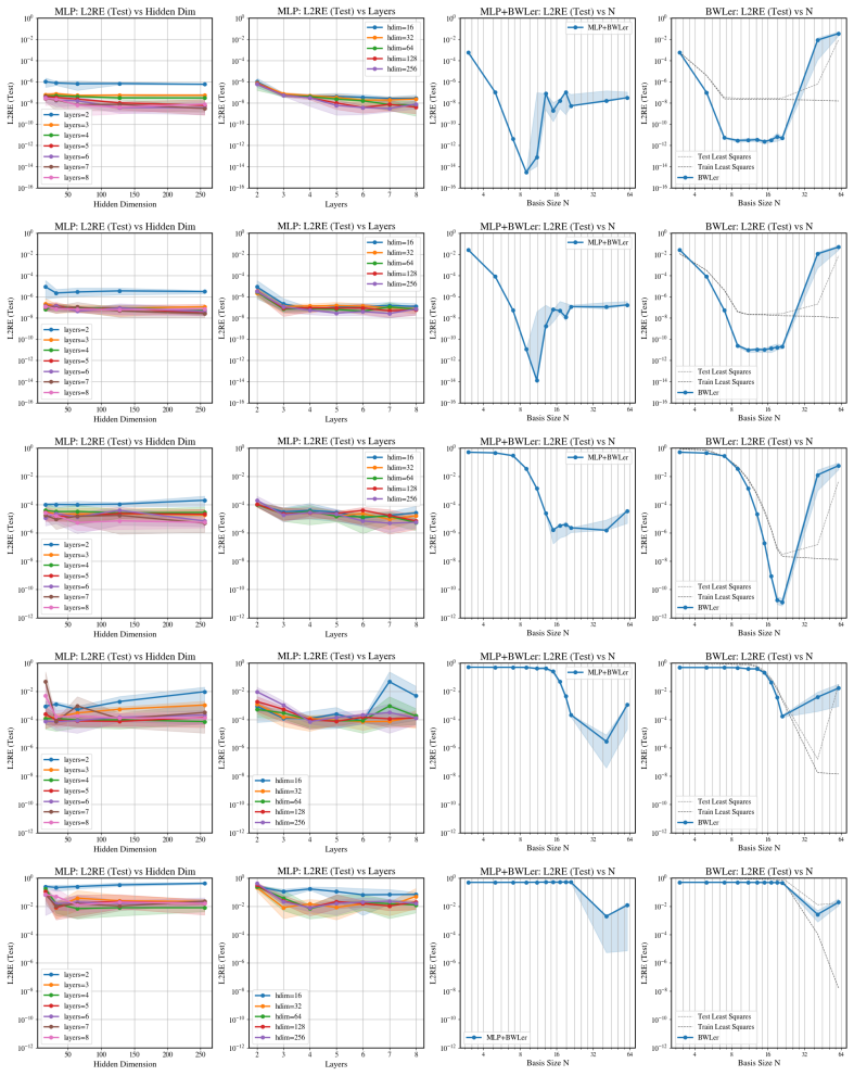
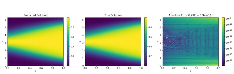
The central claim is that the standard MLP architecture itself imposes a fundamental bottleneck: even on 1-D interpolation without any PDE terms, MLPs with $O(10^5)$ parameters plateau near $10^{-8}$ relative error, while polynomial interpolants of degree 20--50 reach near-machine precision. BWLer embeds barycentric interpolation into the physics-informed framework, decoupling how a solution is represented (node values on a Chebyshev grid, either explicit or MLP-generated) from how derivatives are computed (spectral DCT or finite differences). Theorem 5.1 characterizes the resulting error for linear PDEs as a sum of an expressivity gap $O(\rho^{-N})$, a misspecification gap $O(N^{-(k+1-d)})$ from finite-difference surrogates, and an optimization gap $\exp(-t/\kappa^2)$, and the paper identifies two precision-conditioning tradeoffs: raising $N$ improves expressivity but worsens conditioning, and switching from spectral to finite-difference derivatives improves conditioning but worsens misspecification. Empirically, explicit BWLer with a second-order optimizer achieves near-machine precision ($2\times10^{-13}$ to $1.3\times10^{-11}$ relative error) on convection, reaction, and wave equations, and matches standard PINN precision on Burgers and irregular-geometry Poisson problems, albeit at higher training cost.
Load-bearing premise
The proof of the tradeoff bound assumes that the error from approximating the PDE operator stays controlled by the interpolation residual times the Lebesgue constant, with no further amplification from the inverse of the discretized operator whose condition number grows like $N^{2d}$; if that inverse amplifies the residual, the claimed full characterization of the tradeoff would need an extra stability factor.
Editorial extensions
If this is right
- Physics-informed networks can reach near-machine precision on smooth PDEs without abandoning the PINN loss, as long as the solution is represented polynomially instead of by an MLP.
- Adding BWLer as a hat over an existing MLP is a drop-in precision boost that works with first-order optimizers such as Adam, improving benchmark $\ell^2$ relative errors by up to $1800\times$.
- The tradeoff theorem gives a selection rule: use spectral derivatives when smoothness allows large $N$, and finite-difference stencils when conditioning or convergence speed matters more.
- Explicit BWLer's high precision comes with real costs, longer training and second-order optimization, so the results are a proof of concept for the precision ceiling rather than a runtime-competitive solver.
- Stiff and non-smooth problems (Burgers, irregular Poisson) are not helped by the barycentric representation, which inherits the limits of spectral methods.
Reading between the lines
- If the MLP bottleneck is architectural, other globally smooth representations (Fourier features, tensor-product splines, or wavelets) should show similar precision lifts when paired with spectral differentiation; the paper tests only barycentric polynomials, so this is a testable extension.
- The error decomposition suggests that domain decomposition or element-wise BWLer could relax the $N^{2d}$ conditioning growth while keeping spectral accuracy, a natural next step the paper does not pursue.
- The precision results function as existence proofs: they show the ceiling is liftable, but time-to-solution comparisons against classical spectral solvers would settle whether the framework has standing operational value.
Editorial analysis
A structured set of objections, weighed in public.
Referee Report
Summary. The paper introduces BWLer, a barycentric polynomial interpolation layer that can either replace the MLP in a PINN (explicit BWLer) or be placed on top of an MLP (BWLer-hatted MLP). The central claims are: (i) MLPs have a precision bottleneck that is architectural rather than purely due to PDE ill-conditioning, (ii) BWLer improves conditioning and accuracy on benchmark PDEs, and (iii) for linear PDEs, the paper provides a full theoretical characterization of a precision-conditioning tradeoff, Theorem 5.1, with an error decomposition into expressivity, misspecification, and optimization terms. The empirical section reports large L2RE improvements on convection, reaction, and wave equations, including near-machine-precision results when explicit BWLer is trained with Nyström-Newton-CG.
Significance. If the theoretical characterization were correct, the paper would make a valuable contribution: it cleanly separates representation from differentiation in PINNs, identifies an empirical MLP precision plateau, and demonstrates that a classical barycentric representation can be embedded in a physics-informed learning framework to reach near-machine precision on smooth problems. The paper is also commendable for releasing code and providing detailed appendix material with pseudocode and experimental configurations. However, the formal error decomposition in Theorem D.8 has a proof gap in the bias term that is load-bearing for the claimed tradeoff, so the theoretical contribution is not yet established.
major comments (1)
- [Appendix D.2, Theorem D.8, Eq. (9)] The bias/misspecification bound is not justified. In proof step 2, the paper states that interpolating the nodal residuals off the grid gives ||eu - u*||∞ ≤ Λ_N max_i |r_i|. This is invalid: the error polynomial e = eu - u* does not have nodal values equal to the residual vector r_i; rather, its nodal values solve A e_nodes = r, where A is the collocation matrix. A correct bound requires a factor of ||A^{-1}||, e.g. ||e_nodes||∞ ≤ ||A^{-1}||∞ ||r||∞. The paper itself states in Section 5.2 that for spectral collocation of a d-th order operator κ2(A) = O(N^{2d}), so the missing inverse factor can grow polynomially in N and changes the asymptotic order of the bias term. Consequently, Corollary D.9's claim of a pure O(N^{-(k+1-d)}) misspecification gap is not established, and the precision-conditioning tradeoff stated in Theorem 5.1 is not proven. Because the theorem is presented as the paper's full characterization and Section 5.2 uses this tradeoff to justify derivative-stencil choices, this gap is load-bearing and needs to be repaired, either by including the stability factor and re-deriving the scaling, or by restricting the theorem to settings where the factor is controlled.
minor comments (6)
- [Section 3.2 / Abstract] The phrase "fundamental bottleneck" overstates what the experiments show: Figure 2 demonstrates a plateau for tanh MLPs trained with Adam on a specific 1-D interpolation task, not a proven lower bound over all MLP architectures and optimizers. Please soften to "empirical bottleneck" or provide a formal lower bound.
- [Appendix A.1] The claim that the authors are not aware of any PINN approach reaching machine-precision solutions appears to conflict with reference [10], whose title explicitly mentions "toward machine precision" for PDEs with deep neural nets. Please reconcile this claim with that reference.
- [Table 2] The table caption should state explicitly that the comparisons are not time- or parameter-matched; this fact is mentioned in the main text but should be visible in the table itself to avoid misinterpretation.
- [Section 4 / Section 5] The notation is inconsistent: the paper uses both "BWL ER" and "BWLER" throughout. Please pick one form and use it consistently.
- [Theorem 5.1 / Corollary D.9] There are minor typos, including "Cheybshev" instead of "Chebyshev" in Theorem 5.1's statement, and the bias term in Corollary D.9 is written both as O(N^{-(k+1-d)}) and eO(N^{-(k+1-d)}); please make the notation consistent and include the explicit Λ_N factor.
- [Section 5.2] The headline high-precision results are obtained with Nyström-Newton-CG, while Theorem 5.1 analyzes gradient descent on a quadratic loss; the paper should state clearly that the theorem does not directly analyze NNCG and that the connection is motivational rather than a formal convergence guarantee for the method used in Table 2.
Circularity Check
No circular dependency: BWLer's precision-conditioning results rest on external classical bounds and direct benchmark measurements; the Appendix D.2 gap is a proof-stability issue, not circularity.
full rationale
The claimed derivation chain for BWLer is not circular. The expressivity terms in Theorems 4.1 and 5.1 are the classical Chebyshev/Bernstein-ellipse bounds (Theorem 2.2, from [33,4]); the optimization terms are the standard gradient-descent rate for quadratic least-squares losses from [5]; the misspecification term in Corollary D.9 is the classical finite-difference truncation estimate from [13]; and the conditioning scalings kappa_2(G)=O(1) and kappa_2(A)=O(N^{2d}) come from external approximation-theory sources [33,32]. None of these inputs presuppose the near-machine-precision outcomes reported in Tables 1-2. The high-precision results are direct empirical L2RE measurements against analytical solutions on benchmark PDEs (convection, reaction, wave, Burgers, Poisson); no parameter is fitted to a subset and then reported as a prediction of a closely related quantity. The only reference sharing authors with the present paper is [24], a Transformer least-squares precision study cited in Related Work as context; it is not load-bearing for the BWLer construction or the theorems. One caveat is a proof gap, not a circularity: in Theorem D.8, the bias step bounds ||eu-u*||_inf by the Lebesgue constant times the nodal residual, but e := eu-u* satisfies A e = r at the nodes, so a rigorous bound would need ||A^{-1}||. Since the paper itself notes kappa_2(A)=O(N^{2d}), the missing factor could strengthen the bias term's N-dependence. This is a correctness/stability concern with the 'full characterization' claim, not a reduction of the result to its inputs. Accordingly, the circularity score is 0.
Assumptions & free parameters
free parameters (4)
- Grid sizes (N_t, N_x) for explicit BWLer =
Convection c=40: (81,80); c=80: (161,160); Reaction: (81,81); Wave: (41,41); Burgers: (321,321); Poisson: (51,51)
- NNCG preconditioner rank and CG iterations =
Rank 1000 with 100-1000 CG steps for convection/wave/Poisson/Burgers; rank 16 with 16 CG steps for reaction
- Finite-difference stencil for Burgers time derivative =
1st-order, 3-point stencil
- BWLer grid size N in interpolation experiments =
N in {20,...,26} for BWLer-hat and explicit BWLer
assumptions (4)
- domain assumption The PDE solution extends analytically to a Bernstein ellipse with ρ>1
- domain assumption CGL collocation matrix condition number scales as κ2(A)=O(N^{2d}) for d-th order operators
- domain assumption Nodal collocation at the Chebyshev nodes is sufficient to enforce the PDE
- standard math Empirical Gram concentration via matrix Bernstein (Lemma D.3)
Cite this review
Pith. "Pith review of BWLer: Barycentric Weight Layer Elucidates a Precision-Conditioning Tradeoff for PINNs." pith.science (2026). https://pith.science/paper/5BERCS5P
@misc{pith2026250623024,
  author       = {Pith},
  title        = {Pith review of: BWLer: Barycentric Weight Layer Elucidates a Precision-Conditioning Tradeoff for PINNs},
  year         = {2026},
  howpublished = {\url{https://pith.science/paper/5BERCS5P}},
  note         = {Machine review of arXiv:2506.23024}
}
read the original abstract
Physics-informed neural networks (PINNs) offer a flexible way to solve partial differential equations (PDEs) with machine learning, yet they still fall well short of the machine-precision accuracy many scientific tasks demand. In this work, we investigate whether the precision ceiling comes from the ill-conditioning of the PDEs or from the typical multi-layer perceptron (MLP) architecture. We introduce the Barycentric Weight Layer (BWLer), which models the PDE solution through barycentric polynomial interpolation. A BWLer can be added on top of an existing MLP (a BWLer-hat) or replace it completely (explicit BWLer), cleanly separating how we represent the solution from how we take derivatives for the PDE loss. Using BWLer, we identify fundamental precision limitations within the MLP: on a simple 1-D interpolation task, even MLPs with O(1e5) parameters stall around 1e-8 RMSE -- about eight orders above float64 machine precision -- before any PDE terms are added. In PDE learning, adding a BWLer lifts this ceiling and exposes a tradeoff between achievable accuracy and the conditioning of the PDE loss. For linear PDEs we fully characterize this tradeoff with an explicit error decomposition and navigate it during training with spectral derivatives and preconditioning. Across five benchmark PDEs, adding a BWLer on top of an MLP improves RMSE by up to 30x for convection, 10x for reaction, and 1800x for wave equations while remaining compatible with first-order optimizers. Replacing the MLP entirely lets an explicit BWLer reach near-machine-precision on convection, reaction, and wave problems (up to 10 billion times better than prior results) and match the performance of standard PINNs on stiff Burgers' and irregular-geometry Poisson problems. Together, these findings point to a practical path for combining the flexibility of PINNs with the precision of classical spectral solvers.
Figures


Figures from the paper (21 more)




Reference graph
Works this paper leans on
-
[1]
Battles, Z. and Trefethen, L. N. An extension of matlab to continuous functions and operators. SIAM Journal on Scientific Computing, 25(5):1743–1770, 2004
work page 2004
-
[2]
Berman, J. and Peherstorfer, B. Randomized sparse neural galerkin schemes for solving evolution equations with deep networks. Advances in Neural Information Processing Systems, 36:4097– 4114, 2023
work page 2023
-
[3]
Berrut, J.-P. and Trefethen, L. N. Barycentric lagrange interpolation. SIAM Review, 46(3): 501–517, 2004. doi: 10.1137/S0036144502417715. URL https://doi.org/10.1137/ S0036144502417715
-
[4]
Boyd, J. P. Chebyshev & Fourier Spectral Methods. Lecture Notes in Engineering. Springer Berlin, Heidelberg, Berlin, Heidelberg, 1 edition, 1989. ISBN 978-3-540-51487-9
work page 1989
-
[5]
Boyd, S. P. and Vandenberghe, L.Convex optimization. Cambridge university press, 2004
work page 2004
-
[6]
Brunton, S. L. and Kutz, J. N.Data-driven science and engineering: Machine learning, dynamical systems, and control. Cambridge University Press, 2022
work page 2022
-
[7]
L., Nathan Kutz, J., Manohar, K., Aravkin, A
Brunton, S. L., Nathan Kutz, J., Manohar, K., Aravkin, A. Y ., Morgansen, K., Klemisch, J., Goebel, N., Buttrick, J., Poskin, J., Blom-Schieber, A. W., et al. Data-driven aerospace engineering: reframing the industry with machine learning.Aiaa Journal, 59(8):2820–2847, 2021
work page 2021
-
[8]
Y ., Quarteroni, A., and Zang, T
Canuto, C., Hussaini, M. Y ., Quarteroni, A., and Zang, T. A.Spectral methods, volume 285. Springer, 2006
work page 2006
Show all 43 references
-
[9]
Chen, H., Wu, R., Grinspun, E., Zheng, C., and Chen, P. Y . Implicit neural spatial representations for time-dependent pdes. In International Conference on Machine Learning, pp. 5162–5177. PMLR, 2023. 10
2023
-
[10]
Teng: Time-evolving natural gradient for solving pdes with deep neural nets toward machine precision
Chen, Z., McCarran, J., Vizcaino, E., Soljaˇci´c, M., and Luo, D. Teng: Time-evolving natural gradient for solving pdes with deep neural nets toward machine precision. arXiv preprint arXiv:2404.10771, 2024
2024 arXiv
-
[11]
Cox, S. M. and Matthews, P. C. Exponential time differencing for stiff systems. Journal of Computational Physics, 176(2):430–455, 2002
2002
-
[12]
Evans, L. C. Partial Differential Equations, volume 19 of Graduate Studies in Mathematics. American Mathematical Society, Providence, Rhode Island, 2 edition, 2010. doi: 10.1090/gsm/ 019
2010 doi
-
[13]
Generation of finite difference formulas on arbitrarily spaced grids.Mathematics of computation, 51(184):699–706, 1988
Fornberg, B. Generation of finite difference formulas on arbitrarily spaced grids.Mathematics of computation, 51(184):699–706, 1988
1988
-
[14]
A practical guide to pseudospectral methods
Fornberg, B. A practical guide to pseudospectral methods. Number 1. Cambridge university press, 1998
1998
-
[15]
Turbulence: the legacy of AN Kolmogorov
Frisch, U. Turbulence: the legacy of AN Kolmogorov. Cambridge university press, 1995
1995
-
[16]
Pinnacle: A comprehensive benchmark of physics-informed neural networks for solving pdes,
Hao, Z., Yao, J., Su, C., Su, H., Wang, Z., Lu, F., Xia, Z., Zhang, Y ., Liu, S., Lu, L., and Zhu, J. Pinnacle: A comprehensive benchmark of physics-informed neural networks for solving pdes,
-
[17]
J.The finite element method: linear static and dynamic finite element analysis
Hughes, T. J.The finite element method: linear static and dynamic finite element analysis. Courier Corporation, 2003
2003
-
[18]
Optimizing a discrete loss (odil) to solve forward and inverse problems for partial differential equations using machine learning tools
Karnakov, P., Litvinov, S., and Koumoutsakos, P. Optimizing a discrete loss (odil) to solve forward and inverse problems for partial differential equations using machine learning tools. arXiv preprint arXiv:2205.04611, 2022
2022 arXiv
-
[19]
Solving inverse problems in physics by optimizing a discrete loss: Fast and accurate learning without neural networks.PNAS nexus, 3(1): pgae005, 2024
Karnakov, P., Litvinov, S., and Koumoutsakos, P. Solving inverse problems in physics by optimizing a discrete loss: Fast and accurate learning without neural networks.PNAS nexus, 3(1): pgae005, 2024
2024
-
[20]
E., Kevrekidis, I
Karniadakis, G. E., Kevrekidis, I. G., Lu, L., Perdikaris, P., Wang, S., and Yang, L. Physics- informed machine learning. Nature Reviews Physics, 3(6):422–440, 2021
2021
-
[21]
Kingma, D. P. Adam: A method for stochastic optimization.arXiv preprint arXiv:1412.6980, 2014
2014 arXiv
-
[22]
Krishnapriyan, A., Gholami, A., Zhe, S., Kirby, R., and Mahoney, M. W. Characterizing possible failure modes in physics-informed neural networks.Advances in neural information processing systems, 34:26548–26560, 2021
2021
-
[23]
Liu, D. C. and Nocedal, J. On the limited memory bfgs method for large scale optimization. Mathematical programming, 45(1):503–528, 1989
1989
-
[24]
W., Grogan, J., Dugan, O
Liu, J. W., Grogan, J., Dugan, O. M., Rao, A., Arora, S., Rudra, A., and Re, C. Towards learning high-precision least squares algorithms with sequence models. In The Thirteenth International Conference on Learning Representations, 2025. URL https://arxiv.org/ abs/2503.12295
2025 arXiv
-
[25]
L., Gagne, D
McGovern, A., Elmore, K. L., Gagne, D. J., Haupt, S. E., Karstens, C. D., Lagerquist, R., Smith, T., and Williams, J. K. Using artificial intelligence to improve real-time decision-making for high-impact weather. Bulletin of the American Meteorological Society, 98(10):2073–2090, 2017
2017
-
[26]
and Hakim, A
McGreivy, N. and Hakim, A. Weak baselines and reporting biases lead to overoptimism in machine learning for fluid-related partial differential equations.Nature Machine Intelligence, 6 (10):1256–1269, September 2024. ISSN 2522-5839. doi: 10.1038/s42256-024-00897-5. URL http://d...
2024 doi
-
[27]
J., Liu, Z., and Tegmark, M
Michaud, E. J., Liu, Z., and Tegmark, M. Precision machine learning. Entropy, 25(1):175, January 2023. ISSN 1099-4300. doi: 10.3390/e25010175. URL http://dx.doi.org/10. 3390/e25010175. 11
2023 doi
-
[28]
and Molinaro, R
Mishra, S. and Molinaro, R. Estimates on the generalization error of physics-informed neural networks for approximating pdes. IMA Journal of Numerical Analysis, 43(1):1–43, 2023
2023
-
[29]
Raissi, M., Perdikaris, P., and Karniadakis, G. E. Machine learning of linear differential equations using gaussian processes. Journal of Computational Physics, 348:683–693, November 2017. ISSN 0021-9991. doi: 10.1016/j.jcp.2017.07.050. URL http://dx.doi.org/10.1016/j. jcp.2017.07.050
2017 doi
-
[30]
Physics-informed neural networks: A deep learning framework for solving forward and inverse problems involving nonlinear partial differential equations
Raissi, M., Perdikaris, P., and Karniadakis, G. Physics-informed neural networks: A deep learning framework for solving forward and inverse problems involving nonlinear partial differential equations. Journal of Computational Physics, 378:686–707, 2019. ISSN 0021-9991. doi: ht...
2019 doi
-
[31]
Challenges in training pinns: A loss landscape perspective, 2024
Rathore, P., Lei, W., Frangella, Z., Lu, L., and Udell, M. Challenges in training pinns: A loss landscape perspective, 2024. URL https://arxiv.org/abs/2402.01868
2024 arXiv
-
[32]
Trefethen, L. N. Spectral methods in MATLAB. SIAM, 2000
2000
-
[33]
Trefethen, L. N. Approximation Theory and Approximation Practice, Extended Edition. Society for Industrial and Applied Mathematics, Philadelphia, PA, 2019. doi: 10.1137/1.9781611975949. URL https://epubs.siam.org/doi/abs/10.1137/1.9781611975949
2019 doi
-
[34]
Tropp, J. A. User-friendly tail bounds for sums of random matrices.Foundations of computational mathematics, 12:389–434, 2012
2012
-
[35]
High-dimensional probability: An introduction with applications in data science, volume 47
Vershynin, R. High-dimensional probability: An introduction with applications in data science, volume 47. Cambridge university press, 2018
2018
-
[36]
Understanding and mitigating gradient flow pathologies in physics-informed neural networks
Wang, S., Teng, Y ., and Perdikaris, P. Understanding and mitigating gradient flow pathologies in physics-informed neural networks. SIAM Journal on Scientific Computing, 43(5):A3055–A3081, 2021
2021
-
[37]
An expert’s guide to training physics- informed neural networks, 2023
Wang, S., Sankaran, S., Wang, H., and Perdikaris, P. An expert’s guide to training physics- informed neural networks, 2023. URLhttps://arxiv.org/abs/2308.08468
2023 arXiv
-
[38]
and Lai, C.-Y
Wang, Y . and Lai, C.-Y . Multi-stage neural networks: Function approximator of machine precision, 2023. URL https://arxiv.org/abs/2307.08934
2023 arXiv
-
[39]
Turbulence Modeling for CFD
Wilcox, D. Turbulence Modeling for CFD. Number v. 1 in Turbulence Modeling for CFD. DCW Industries, 2006. ISBN 9781928729082. URL https://books.google.com/books?id= tFNNPgAACAAJ
2006
-
[40]
fixed nodal collocation
Yao, Z., Gholami, A., Keutzer, K., and Mahoney, M. W. Pyhessian: Neural networks through the lens of the hessian. In2020 IEEE international conference on big data (Big data), pp. 581–590. IEEE, 2020. 12 A Related work A.1 High-precision machine learning for PDEs The difficulty...
2020
-
[42]
This term accounts for the gap between the best polynomial ap- proximation to the PDE solution, u∗, and the true solution to the numerical surrogate, eu
Bias/misspecification term. This term accounts for the gap between the best polynomial ap- proximation to the PDE solution, u∗, and the true solution to the numerical surrogate, eu. At each node, ri = (eL−L)u∗(xi), |ri| ≤Muεop(N ). Hence ∥ eAθ∗ −eb∥∞ = maxi|ri|, and interpolat...
-
[43]
This term accounts for the gap between the t-th iterate, u(t) N , and the true solution to the numerical surrogate PDE,eu
Optimization term. This term accounts for the gap between the t-th iterate, u(t) N , and the true solution to the numerical surrogate PDE,eu. Gradient descent on the quadratic loss function yields ∥θ(t) −θ∗∥2 ≤ exp −t/κ2( eA) ∥θ∗∥2. For any x, |u(t) N −eu(x)| = NX j=0 (θ(t) j ...
-
[2023]
URL https://arxiv.org/abs/2306.08827
Reviewed August 6, 2026 · model on record in the stance chip above.
Discussion (0). Sign in to comment.