REVIEW 3 major objections 5 minor 63 references
Generalizing to New Dynamical Systems via Frequency Domain Adaptation
T0 review · 3 major / 5 minor · reviewed 2026-08-07 · deepseek-v4-flash
Pith's one-line read A neural simulator, FNSDA, generalizes to new dynamical systems of the same physical family by adapting in Fourier space, updating about 90 parameters and matching or beating baselines that retune thousands to millions.
desk verdict Genuine but incremental Fourier-domain adaptation method with real parameter efficiency, undermined by a probable Gray-Scott test-parameter error that needs fixing before its headline PDE results are credible. read the letter →
The pith
A machine-rendered reading of the paper's core claim, the machinery that carries it, and where it could break.
The reading
What carries the argument
The object that carries the argument is the mode-partitioned Fourier kernel, a modification of the Fourier Neural Operator layer $K^{(l)}(z^{(l)}) = \mathrm{IFFT}(R^{(l)} \cdot \mathrm{FFT}(z^{(l)}))$. FNSDA inserts a learnable filter $K^{(l)} \in \mathbb{R}^{\hat{k}}$ (trained through a hard sigmoid so its entries approach 0 or 1) that splits the truncated Fourier modes into shared modes $\mathrm{FFT}_s = (1-K^{(l)})\cdot\mathrm{FFT}(z^{(l)})$, multiplied by a frozen weight $R_s^{(l)}$, and environment modes $\mathrm{FFT}_e = K^{(l)}\cdot\mathrm{FFT}(z^{(l)})$, multiplied by $R_e^{(l)} = W_{\mathrm{env}}^{(l)} c_e$. Because the same low-dimensional $c_e$ (dimension 10 or 20) feeds every Fourier layer through the hierarchy, its influence is amplified, so the only parameters updated during adaptation are $c_e$ and the per-environment Swish slopes $\beta_e^{(l)}$; the partition, the shared weights, and the lifting and projection operators remain frozen. Training pairs this with L2 regularization on $c_e$ and a cosine-annealing schedule with warmup, and adaptation initializes from the training-environment averages of $c_e$ and $\beta_e$.
What would settle it
Adapt FNSDA to a test environment whose parameters lie well outside the training range, or whose dynamics enter a qualitatively different regime such as a chaotic one (which the authors state they have not tested). If updating only $c_e$ and $\beta_e$ cannot push the forecast error substantially below the frozen-network baseline, the linear-transfer premise fails. A sharper probe is spectral: estimate the environment-specific Fourier kernel difference of a held-out environment from data and check whether it is approximately low-rank and lies in the span of $W_{\mathrm{env}}^{(l)}$; the paper does not report such a diagnostic.
Extended reading notes
Core claim
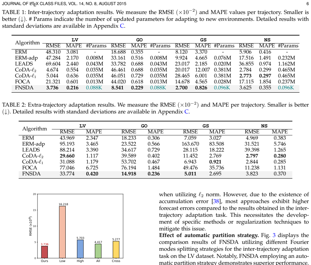
The central claim is that cross-environment transfer in learned simulators is a low-dimensional, linear problem once the dynamics are viewed in the frequency domain: the differences between environments can be expressed as $R_e^{(l)} = W_{\mathrm{env}}^{(l)} c_e$, a learned linear map of a shared latent context vector applied to a subset of Fourier modes, while a second subset of modes carries dynamics common to all environments and stays untouched during adaptation. FNSDA learns which modes belong to which subset through a hard-sigmoid filter $K^{(l)}$ trained on the source environments, and at test time only $c_e$ and the Swish parameter $\beta_e^{(l)}$ are updated, initialized at their training averages. The paper reports that this scheme yields the smallest inter-trajectory adaptation error on the Lotka-Volterra, glycolytic-oscillator, and Gray-Scott systems, results second only to the CoDA family on Navier-Stokes, and best-or-competitive performance in extra-trajectory forecasting, with two to four orders of magnitude fewer updated parameters than the baselines and faster convergence.
Load-bearing premise
The paper assumes that every unseen environment of a given equation family differs from the training environments in a way that a single linear map of a small context vector can express, applied to the same set of frequency modes the network learned to treat as environment-specific; if a new environment's discrepancy is not low-rank and linear in Fourier space, or occupies modes the learned partition did not reserve, no amount of adapting $c_e$ can represent it.
Editorial extensions
If this is right
- A single pretrained FNSDA simulator can adapt to an unseen environment from one trajectory, since adaptation reduces to inferring the context vector and one activation slope per layer.
- Adaptation cost is set by the context dimension rather than the network size, so the method works where full fine-tuning is impractical, such as partially reconfigurable edge hardware.
- The learned mode partition beats manual splits at every tested ratio (4:1 through 1:4), so which modes are environment-specific is data-dependent rather than simply high- or low-frequency.
- Because only about 90 parameters change, convergence during adaptation is fast: roughly 1,200 iterations for one-shot tasks and about 100 for extra-trajectory tasks on the Lotka-Volterra system.
- Best-or-competitive results hold across ODE families (Lotka-Volterra, glycolytic oscillations) and PDE families (Gray-Scott, Navier-Stokes), indicating the mechanism is not tied to a single equation form.
Reading between the lines
- A direct test the paper does not run would be to estimate the true frequency-domain discrepancy of held-out environments from data and compare its rank with the capacity of $W_{\mathrm{env}}^{(l)} c_e$; if the discrepancy is high-rank or falls on modes the learned partition did not reserve, the method's ceiling could be identified before deployment.
- If the linear-context mechanism is as general as claimed, the same conditioning could be grafted onto other operator learners, such as graph-based or transformer-based simulators, by applying $W_{\mathrm{env}} c_e$ to their spectral or latent channels; that would reveal whether the claim is specific to Fourier space or about low-rank environment conditioning generally.
- The one extrapolation experiment in Fig. 4(b) suggests the method tolerates non-interpolatable environmental parameters, but the paper tests only Lotka-Volterra and does not approach bifurcations or regime changes; a chaotic or bistable family would be a more adversarial test, and the authors themselves flag chaotic systems as untested.
- The stated efficiency of 88 to 96 parameters counts only $c_e$ and $\beta_e$; a deployment-oriented accounting would also include the cost of inferring $c_e$ from observations through gradient steps on the frozen network, which the paper's convergence curves suggest is small but not zero.
Editorial analysis
A structured set of objections, weighed in public.
Referee Report
Summary. The paper proposes FNSDA, a Fourier-domain adaptation method for learning simulators that generalize to new dynamical systems. FNSDA builds on the Fourier Neural Operator (FNO) architecture, learns a hard-sigmoid partition of Fourier modes into shared and environment-specific groups, and conditions the environment-specific weights on a low-dimensional context vector c_e. At test time, only c_e and the Swish activation slopes are updated, giving 88-96 updated parameters per test environment. The method is evaluated on two ODE families (Lotka-Volterra and yeast glycolysis) and two PDE families (Gray-Scott and Navier-Stokes) under inter-trajectory and extra-trajectory adaptation. The reported results show large gains over the compared baselines on GO and GS, competitive results on NS, and much lower adaptation parameter counts.
Significance. If the results hold, FNSDA would be a meaningful contribution to data-driven dynamical-system generalization: it would show that a single Fourier-domain simulator can adapt to unseen environments of the same equation family with a tiny parameter budget, while matching or beating methods that update hundreds of thousands of parameters. The paper has genuine strengths: two complementary evaluation protocols, four system families, careful ablations of the partition strategy and training techniques, parameter-sensitivity analyses, convergence curves, and an explicit limitations section. However, two issues currently block full confidence: the Gray-Scott benchmark as described appears to evaluate a qualitatively different parameter regime than the training regime, and the baselines share an MLP backbone while FNSDA uses an FNO, so the headline gains are not cleanly attributable to the proposed adaptation mechanism.
major comments (3)
- [Appendix B.1; Tables 1-2] The Gray-Scott test environments are defined with k in {0.59, 0.61} while the training environments use k in {0.058, 0.062}; this is a factor-of-ten jump, and the caption of Figs. 8-9 confirms that the visualized test case uses (F,k)=(0.33,0.61). In the Gray-Scott PDE, the v-equation contains the term (F+k)v, so with k=0.61 the linear decay is an order of magnitude faster than in training and the test dynamics are far outside the pattern-forming regime of the training family. The GS rows in Tables 1 and 2 contain some of the largest reported gaps (inter-trajectory RMSE 2.700 for FNSDA vs 20.017 for CoDA-l2; extra-trajectory 5.011 vs 6.943 for CoDA-l1), so the four-family claim currently rests on a benchmark setup that cannot be attributed to the proposed frequency-domain adaptation mechanism. Please rerun the GS experiments with consistent parameters (e.g., k=0.059/0.061) or otherwise justify the regime, and provide a versioned code release so the generated data can be checked.
- [§4.1 Baselines; Tables 1-2] All compared baselines are implemented with the architecture used in [15], which is a temporal-domain MLP dynamics model, whereas FNSDA uses an FNO with Fourier layers. The main tables therefore conflate two differences: the model class (FNO vs MLP) and the adaptation mechanism (Fourier-mode partition with low-dimensional conditioning vs full or contextual fine-tuning). A large part of the reported gains could come from FNO's stronger per-environment fitting rather than from the proposed partition-and-conditioning idea; the in-domain results in Table 6, where FNSDA also beats the baselines, are consistent with an architecture effect. To support the central claim, please isolate the contribution by adding, for example, an FNO baseline that is fine-tuned under the same adaptation protocol (updating all parameters) and/or an MLP instantiation of FNSDA's conditioning mechanism, and report both in the main comparison.
- [§3.2, Eqs. (5)-(6); Fig. 4(b)] The transfer mechanism assumes that a single learned partition K^(l), and a linear conditioning map R_e^(l)=W_env^(l)c_e trained on the known environments, can represent the discrepancies of unseen environments. The paper validates this only indirectly through end-to-end accuracy on the four benchmarks, and the only extrapolation test (Fig. 4b on LV) is a single case. Because adaptation updates only c_e and the Swish slopes, a direct validation is needed: for example, compare the fixed K^(l) with a partition fitted on a test environment, or measure how well the low-rank approximation W_env^(l)c_e reconstructs the test-environment dynamics. Without such evidence, the claim that the method 'identifies' shareable versus environment-specific modes for new systems is supported by outcome rather than by inspection of the proposed mechanism.
minor comments (5)
- [§4.1] The text says 'd_c=10 for the LV and NV datasets'; 'NV' should be 'NS'.
- [Appendix C.2] The phrase 'varying victory' should be 'varying viscosity'.
- [Appendix C.4] The ablation table is captioned 'Table E' but is numbered Table 11; please number it consistently and reference it correctly in the text.
- [Tables 1-2] The main-text tables omit standard deviations even though they are available in Appendix C.1; some claimed advantages, such as the NS row of Table 2, are within one standard deviation, so the main text should either include the error bars or explicitly point to the appendix rows.
- [Abstract and code link] The GitHub link has no commit hash or release tag; a pinned version would materially improve reproducibility, especially given the Gray-Scott parameter inconsistency described above.
Circularity Check
No significant circularity: the central generalization claims are evaluated against held-out trajectories and future-time predictions, with the adaptation parameters inferred from data rather than constructed from the target outputs.
full rationale
FNSDA's derivation chain is self-contained with respect to its empirical claims. The environment-specific map R_e^(l) = W_env^(l) c_e is learned from training environments, and at test time only the low-dimensional c_e and Swish parameters beta_e are updated using observed trajectories from the unseen environment. Predictions are then made on held-out trajectories of the same environment (inter-trajectory) or on future time points not used in adaptation (extra-trajectory). This is genuine held-out evaluation, not a fitted parameter renamed as a prediction. The Fourier-mode partition K^(l) is trained on known environments and then applied to unseen environments; whether that inductive bias holds is an assumption whose validity is tested empirically, not an identity forced by construction. The only self-citations are [34] and [36] in the related-work discussion, and they are not load-bearing for the method's correctness or for the generalization results. The Gray-Scott test-parameter discrepancy noted in Appendix B.1 (k in {0.59, 0.61} for test environments versus k in {0.058, 0.062} for training environments) is a potentially serious experimental-validity concern, but it is not a circularity: it does not show that any prediction is equivalent to an input by construction. The paper does not invoke an author-specific uniqueness theorem, and no step reduces to redefining the output as the input. Therefore no circular step is identified, and the circularity score is 0.
Assumptions & free parameters
free parameters (4)
- c_e (environment context vector) =
d_c = 10 (LV, NS), 20 (GO, GS); learned per environment
- lambda (regularization coefficient) =
1e-4
- k_hat (truncated modes) and layer count L =
k_hat=10, L=2 (LV, GO); k_hat=12, L=4 (GS, NS)
- beta_e (Swish activation slope) =
learned per environment per layer
assumptions (5)
- domain assumption All environments share the same family of differential equations and differ only in hidden parameters.
- domain assumption Nonlinear dynamics become approximately linear in Fourier space, so environment discrepancies are representable by linear scaling of a few Fourier modes.
- ad hoc to paper A single learned hard-sigmoid filter K^l, trained on known environments, separates shared from environment-specific modes for unseen environments.
- ad hoc to paper The linear conditioning R_e^l = W_env^l c_e can represent unseen environment dynamics.
- domain assumption Training data come from accurate numerical simulators and are noise-free.
invented entities (1)
-
c_e latent systematic parameter
Cite this review
Pith. "Pith review of Generalizing to New Dynamical Systems via Frequency Domain Adaptation." pith.science (2026). https://pith.science/paper/ZLRG3L2P
@misc{pith2026250700025,
  author       = {Pith},
  title        = {Pith review of: Generalizing to New Dynamical Systems via Frequency Domain Adaptation},
  year         = {2026},
  howpublished = {\url{https://pith.science/paper/ZLRG3L2P}},
  note         = {Machine review of arXiv:2507.00025}
}
read the original abstract
Learning the underlying dynamics from data with deep neural networks has shown remarkable potential in modeling various complex physical dynamics. However, current approaches are constrained in their ability to make reliable predictions in a specific domain and struggle with generalizing to unseen systems that are governed by the same general dynamics but differ in environmental characteristics. In this work, we formulate a parameter-efficient method, Fourier Neural Simulator for Dynamical Adaptation (FNSDA), that can readily generalize to new dynamics via adaptation in the Fourier space. Specifically, FNSDA identifies the shareable dynamics based on the known environments using an automatic partition in Fourier modes and learns to adjust the modes specific for each new environment by conditioning on low-dimensional latent systematic parameters for efficient generalization. We evaluate our approach on four representative families of dynamic systems, and the results show that FNSDA can achieve superior or competitive generalization performance compared to existing methods with a significantly reduced parameter cost. Our code is available at https://github.com/WonderSeven/FNSDA.
Figures


Figures from the paper (8 more)


Reference graph
Works this paper leans on
-
[15]
Generalizing to new physical systems via context-informed dynamics model,
M. Kirchmeyer, Y. Yin, J. Donà, N. Baskiotis, A. Rakotomamonjy, and P . Gallinari, “Generalizing to new physical systems via context-informed dynamics model,” inICML, 2022
work page 2022
-
[1]
Reynolds averaged turbulence modelling using deep neural networks with embedded invariance,
J. Ling, A. Kurzawski, and J. Templeton, “Reynolds averaged turbulence modelling using deep neural networks with embedded invariance,”Journal of Fluid Mechanics, vol. 807, pp. 155–166, 2016. JOURNAL OF LATEX CLASS FILES, VOL. 14, NO. 8, AUGUST 2015 8
work page 2016
-
[2]
Discovering governing equations from data by sparse identification of nonlinear dynami- cal systems,
S. L. Brunton, J. L. Proctor, and J. N. Kutz, “Discovering governing equations from data by sparse identification of nonlinear dynami- cal systems,”PNAS, vol. 113, no. 15, pp. 3932–3937, 2016
work page 2016
-
[3]
Hidden fluid mechanics: Learning velocity and pressure fields from flow vi- sualizations,
M. Raissi, A. Yazdani, and G. E. Karniadakis, “Hidden fluid mechanics: Learning velocity and pressure fields from flow vi- sualizations,”Science, vol. 367, no. 6481, pp. 1026–1030, 2020
work page 2020
-
[4]
Machine learning–accelerated computational fluid dynamics,
D. Kochkov, J. A. Smith, A. Alieva, Q. Wang, M. P . Brenner, and S. Hoyer, “Machine learning–accelerated computational fluid dynamics,”PNAS, vol. 118, no. 21, 2021
work page 2021
-
[5]
Lagrangian fluid simulation with continuous convolutions,
B. Ummenhofer, L. Prantl, N. Thuerey, and V . Koltun, “Lagrangian fluid simulation with continuous convolutions,” inICLR, 2020
work page 2020
-
[6]
J. A. Weyn, D. R. Durran, and R. Caruana, “Can machines learn to predict weather? using deep learning to predict gridded 500- hpa geopotential height from historical weather data,”Journal of Advances in Modeling Earth Systems, vol. 11, no. 8, 2019
work page 2019
-
[7]
J. Pathak, S. Subramanian, P . Harrington, S. Raja, A. Chattopad- hyay, M. Mardani, T. Kurth, D. Hall, Z. Li, K. Azizzadenesheli et al., “Fourcastnet: A global data-driven high-resolution weather model using adaptive fourier neural operators,”arXiv preprint arXiv:2202.11214, 2022
arXiv 2022
Show all 63 references
-
[8]
Inferring halo masses with graph neural networks,
P . Villanueva-Domingo, F. Villaescusa-Navarro, D. Anglés- Alcázar, S. Genel, F. Marinacci, D. N. Spergel, L. Hernquist, M. Vo- gelsberger, R. Dave, and D. Narayanan, “Inferring halo masses with graph neural networks,”The Astrophysical Journal, vol. 935, no. 1, p. 30, 2022
2022
-
[9]
Sparsity in continuous-depth neural networks,
H. Aliee, T. Richter, M. Solonin, I. Ibarra, F. J. Theis, and N. Kilber- tus, “Sparsity in continuous-depth neural networks,” inNeurIPS, 2022
2022
-
[10]
Physics-guided deep learning for dynamical systems: A survey,
R. Wang and R. Yu, “Physics-guided deep learning for dynamical systems: A survey,”arXiv preprint arXiv:2107.01272, 2021
2021 arXiv
-
[11]
Meta-learning dynamics forecast- ing using task inference,
R. Wang, R. Walters, and R. Yu, “Meta-learning dynamics forecast- ing using task inference,”NeurIPS, 2022
2022
-
[12]
Efficient computation of electrograms and ecgs in human whole heart simulations using a reaction- eikonal model,
A. Neic, F. O. Campos, A. J. Prassl, S. A. Niederer, M. J. Bishop, E. J. Vigmond, and G. Plank, “Efficient computation of electrograms and ecgs in human whole heart simulations using a reaction- eikonal model,”Journal of computational physics, vol. 346, 2017
2017
-
[13]
Generalizing to unseen domains: A survey on domain generalization,
J. Wang, C. Lan, C. Liu, Y. Ouyang, T. Qin, W. Lu, Y. Chen, W. Zeng, and P . Yu, “Generalizing to unseen domains: A survey on domain generalization,”TKDE, 2022
2022
-
[14]
Leads: Learning dynamical systems that generalize across envi- ronments,
Y. Yin, I. Ayed, E. de Bézenac, N. Baskiotis, and P . Gallinari, “Leads: Learning dynamical systems that generalize across envi- ronments,”NeurIPS, vol. 34, pp. 7561–7573, 2021
2021
-
[16]
First-order context-based adaptation for generalizing to new dynamical systems,
J. Park, F. Berto, A. Jamgochian, M. Kochenderfer, and J. Park, “First-order context-based adaptation for generalizing to new dynamical systems,” 2023
2023
-
[17]
Sequential latent variable models for few-shot high-dimensional time-series forecasting,
X. Jiang, R. Missel, Z. Li, and L. Wang, “Sequential latent variable models for few-shot high-dimensional time-series forecasting,” in ICLR, 2023
2023
-
[18]
Deep learning and transfer learning for device-free human activity recognition: A survey,
J. Yang, Y. Xu, H. Cao, H. Zou, and L. Xie, “Deep learning and transfer learning for device-free human activity recognition: A survey,”Journal of Automation and Intelligence, 2022
2022
-
[19]
A review of federated meta-learning and its application in cyberspace secu- rity,
F. Liu, M. Li, X. Liu, T. Xue, J. Ren, and C. Zhang, “A review of federated meta-learning and its application in cyberspace secu- rity,”Electronics, vol. 12, no. 15, p. 3295, 2023
2023
-
[20]
An algorithm for the machine calculation of complex fourier series,
J. W. Cooley and J. W. Tukey, “An algorithm for the machine calculation of complex fourier series,”Mathematics of computation, vol. 19, no. 90, pp. 297–301, 1965
1965
-
[21]
Van Loan,Computational frameworks for the fast Fourier transform
C. Van Loan,Computational frameworks for the fast Fourier transform. SIAM, 1992
1992
-
[22]
S. J. Orfanidis,Introduction to signal processing. Prentice-Hall, Inc., 1995
1995
-
[23]
Distribu- tionally robust neural networks,
S. Sagawa, P . W. Koh, T. B. Hashimoto, and P . Liang, “Distribu- tionally robust neural networks,” inICLR, 2020
2020
-
[24]
Statistics of ro- bust optimization: A generalized empirical likelihood approach,
J. C. Duchi, P . W. Glynn, and H. Namkoong, “Statistics of ro- bust optimization: A generalized empirical likelihood approach,” Mathematics of Operations Research, vol. 46, no. 3, pp. 946–969, 2021
2021
-
[25]
The risks of invariant risk minimization,
E. Rosenfeld, P . K. Ravikumar, and A. Risteski, “The risks of invariant risk minimization,” inICLR, 2021
2021
-
[26]
Out-of-distribution generalization via risk extrapolation (rex),
D. Krueger, E. Caballero, J.-H. Jacobsen, A. Zhang, J. Binas, D. Zhang, R. Le Priol, and A. Courville, “Out-of-distribution generalization via risk extrapolation (rex),” inICML, 2021
2021
-
[27]
Domain agnostic learning with disentangled representations,
X. Peng, Z. Huang, X. Sun, and K. Saenko, “Domain agnostic learning with disentangled representations,” inICML, 2019
2019
-
[28]
Gmfad: Towards gen- eralized visual recognition via multilayer feature alignment and disentanglement,
H. Li, S. Wang, R. Wan, and A. C. Kot, “Gmfad: Towards gen- eralized visual recognition via multilayer feature alignment and disentanglement,”TP AMI, vol. 44, no. 3, pp. 1289–1303, 2022
2022
-
[29]
Learning to generalize: Meta-learning for domain generalization,
D. Li, Y. Yang, Y.-Z. Song, and T. M. Hospedales, “Learning to generalize: Meta-learning for domain generalization,” inAAAI, 2018
2018
-
[30]
Domain generalization via model-agnostic learning of semantic features,
Q. Dou, D. Coelho de Castro, K. Kamnitsas, and B. Glocker, “Domain generalization via model-agnostic learning of semantic features,”NeurIPS, vol. 32, pp. 6450–6461, 2019
2019
-
[31]
Generalizing to unseen domains via adversarial data augmentation,
R. Volpi, H. Namkoong, O. Sener, J. C. Duchi, V . Murino, and S. Savarese, “Generalizing to unseen domains via adversarial data augmentation,”NeurIPS, vol. 31, 2018
2018
-
[32]
Domain generalization with mixstyle,
K. Zhou, Y. Yang, Y. Qiao, and T. Xiang, “Domain generalization with mixstyle,” inICLR, 2021
2021
-
[33]
Regular- izing deep networks with semantic data augmentation,
Y. Wang, G. Huang, S. Song, X. Pan, Y. Xia, and C. Wu, “Regular- izing deep networks with semantic data augmentation,”TP AMI, vol. 44, no. 7, pp. 3733–3748, 2022
2022
-
[34]
Generalizing to evolving domains with latent structure-aware sequential autoencoder,
T. Qin, S. Wang, and H. Li, “Generalizing to evolving domains with latent structure-aware sequential autoencoder,” inICML, 2022
2022
-
[35]
Training for the future: A simple gradient interpolation loss to generalize along time,
A. Nasery, S. Thakur, V . Piratla, A. De, and S. Sarawagi, “Training for the future: A simple gradient interpolation loss to generalize along time,”NeurIPS, vol. 34, pp. 19 198–19 209, 2021
2021
-
[36]
Evolving domain generalization via latent structure-aware sequential autoencoder,
T. Qin, S. Wang, and H. Li, “Evolving domain generalization via latent structure-aware sequential autoencoder,”TP AMI, vol. 45, no. 12, pp. 14 514–14 527, 2023
2023
-
[37]
Neural ordinary differential equations,
R. T. Chen, Y. Rubanova, J. Bettencourt, and D. K. Duvenaud, “Neural ordinary differential equations,”NeurIPS, vol. 31, 2018
2018
-
[38]
Learning to simulate complex physics with graph networks,
A. Sanchez-Gonzalez, J. Godwin, T. Pfaff, R. Ying, J. Leskovec, and P . Battaglia, “Learning to simulate complex physics with graph networks,” inICML, 2020, pp. 8459–8468
2020
-
[39]
Learning mesh-based simulation with graph networks,
T. Pfaff, M. Fortunato, A. Sanchez-Gonzalez, and P . Battaglia, “Learning mesh-based simulation with graph networks,” inICLR, 2021
2021
-
[40]
Learning dynamical systems from data: An introduction to physics-guided deep learning,
R. Yu and R. Wang, “Learning dynamical systems from data: An introduction to physics-guided deep learning,”PNAS, vol. 121, no. 27, p. e2311808121, 2024
2024
-
[41]
Scaling learning algorithms towards ai,
Y. Bengio, Y. LeCunet al., “Scaling learning algorithms towards ai,”Large-scale kernel machines, vol. 34, no. 5, pp. 1–41, 2007
2007
-
[42]
Learning long term dependencies via fourier recurrent units,
J. Zhang, Y. Lin, Z. Song, and I. Dhillon, “Learning long term dependencies via fourier recurrent units,” inICML, 2018
2018
-
[43]
Fast training of convolu- tional networks through ffts,
M. Mathieu, M. Henaff, and Y. LeCun, “Fast training of convolu- tional networks through ffts,” inICLR, 2014
2014
-
[44]
Fnet: Mixing tokens with fourier transforms,
J. Lee-Thorp, J. Ainslie, I. Eckstein, and S. Ontanon, “Fnet: Mixing tokens with fourier transforms,” inNAACL, 2022
2022
-
[45]
Implicit neural representations with periodic activation func- tions,
V . Sitzmann, J. Martel, A. Bergman, D. Lindell, and G. Wetzstein, “Implicit neural representations with periodic activation func- tions,”NeurIPS, vol. 33, pp. 7462–7473, 2020
2020
-
[46]
Robustperiod: Robust time-frequency mining for multiple periodicity detection,
Q. Wen, K. He, L. Sun, Y. Zhang, M. Ke, and H. Xu, “Robustperiod: Robust time-frequency mining for multiple periodicity detection,” inSIGMOD, 2021, pp. 2328–2337
2021
-
[47]
Fourier neural operator for parametric partial differential equations,
Z. Li, N. B. Kovachki, K. Azizzadenesheli, B. liu, K. Bhattacharya, A. Stuart, and A. Anandkumar, “Fourier neural operator for parametric partial differential equations,” inICLR, 2021
2021
-
[48]
Learning chaotic dynamics in dissipative systems,
Z. Li, M. Liu-Schiaffini, N. Kovachki, K. Azizzadenesheli, B. Liu, K. Bhattacharya, A. Stuart, and A. Anandkumar, “Learning chaotic dynamics in dissipative systems,” inNeurIPS, vol. 35, 2022
2022
-
[49]
Factorized fourier neural operators,
A. Tran, A. Mathews, L. Xie, and C. S. Ong, “Factorized fourier neural operators,” inICLR, 2023
2023
-
[50]
On universal approx- imation and error bounds for fourier neural operators,
N. Kovachki, S. Lanthaler, and S. Mishra, “On universal approx- imation and error bounds for fourier neural operators,”JMLR, vol. 22, no. 290, pp. 1–76, 2021
2021
-
[51]
H. J. Nussbaumer and H. J. Nussbaumer,The fast Fourier transform. Springer, 1981
1981
-
[52]
Searching for activation functions,
P . Ramachandran, B. Zoph, and Q. V . Le, “Searching for activation functions,” 2018
2018
-
[53]
Predicting physics in mesh-reduced space with temporal attention,
X. Han, H. Gao, T. Pfaff, J.-X. Wang, and L. Liu, “Predicting physics in mesh-reduced space with temporal attention,” inICLR, 2022
2022
-
[54]
A. J. Lotka,Elements of physical biology. Williams & Wilkins, 1925
1925
-
[55]
Efficient inference of parsi- monious phenomenological models of cellular dynamics using s- systems and alternating regression,
B. C. Daniels and I. Nemenman, “Efficient inference of parsi- monious phenomenological models of cellular dynamics using s- systems and alternating regression,”PloS one, vol. 10, no. 3, 2015
2015
-
[56]
Complex patterns in a simple system,
J. E. Pearson, “Complex patterns in a simple system,”Science, vol. 261, no. 5118, pp. 189–192, 1993
1993
-
[57]
On the effect of the internal friction of fluids on the motion of pendulums,
G. G. Stokes, “On the effect of the internal friction of fluids on the motion of pendulums,”T ransactions of the Cambridge Philosophical Society, vol. 9, pp. 8–106, 1851
-
[58]
Statistical learning theory wiley,
V . Vapnik, “Statistical learning theory wiley,”New Y ork, 1998. JOURNAL OF LATEX CLASS FILES, VOL. 14, NO. 8, AUGUST 2015 9
1998
-
[59]
Automatic differ- entiation in pytorch,
A. Paszke, S. Gross, S. Chintala, G. Chanan, E. Yang, Z. DeVito, Z. Lin, A. Desmaison, L. Antiga, and A. Lerer, “Automatic differ- entiation in pytorch,” inNIPS Workshop, 2017
2017
-
[60]
Adam: A method for stochastic optimiza- tion,
D. P . Kingma and J. Ba, “Adam: A method for stochastic optimiza- tion,” inICLR, 2015
2015
-
[61]
Fpga dynamic and partial reconfigura- tion: A survey of architectures, methods, and applications,
K. Vipin and S. A. Fahmy, “Fpga dynamic and partial reconfigura- tion: A survey of architectures, methods, and applications,”ACM Computing Surveys (CSUR), vol. 51, no. 4, pp. 1–39, 2018
2018
-
[62]
Transform once: Efficient operator learning in frequency domain,
M. Poli, S. Massaroli, F. Berto, J. Park, T. Dao, C. Ré, and S. Er- mon, “Transform once: Efficient operator learning in frequency domain,”NeurIPS, vol. 35, pp. 7947–7959, 2022
2022
-
[63]
Physics perception in sloshing scenes with guaranteed thermo- dynamic consistency,
B. Moya, A. Badías, D. González, F. Chinesta, and E. Cueto, “Physics perception in sloshing scenes with guaranteed thermo- dynamic consistency,”TP AMI, vol. 45, no. 2, pp. 2136–2150, 2023. JOURNAL OF LATEX CLASS FILES, VOL. 14, NO. 8, AUGUST 2015 10 Supplementary Materials Tab...
2023
Reviewed August 7, 2026 · model on record in the stance chip above.
Discussion (0). Sign in to comment.