REVIEW 2 major objections 6 minor 55 references
Gradient Short-Circuit: Efficient Out-of-Distribution Detection via Feature Intervention
T0 review · 2 major / 6 minor · reviewed 2026-08-06 · deepseek-v4-flash
Pith's one-line read Gradient Short-Circuit zeros the few most gradient-sensitive feature coordinates, pushing OOD confidence below threshold while leaving ID accuracy nearly unchanged.
desk verdict The core idea is worth a look, but the ImageNet tables have a copied-baseline problem that makes the headline results unverifiable as printed. read the letter →
The pith
A machine-rendered reading of the paper's core claim, the machinery that carries it, and where it could break.
The reading
What carries the argument
The central object is the gradient vector $g = \nabla_F [y]_c$, the sensitivity of the predicted logit to each coordinate of the high-level feature vector. The intervention is a mask on the coordinates with the largest $|g_i|$, giving $F' = F \odot m$ and $\Delta F = F' - F$. The efficiency device is the local first-order Taylor formula $y' \approx y + (\nabla_F y)^\top \Delta F$, which reuses the backward pass instead of rerunning the classification head; the paper's error bound is $\|y'_{\mathrm{exact}} - y'_{\mathrm{approx}}\| \le \tfrac12 L_{\mathrm{smooth}} \|\Delta F\|^2$.
What would settle it
Two checks would settle the matter: measure the gradient concentration (for example, TopKRatio(50)) on a near-OOD pair such as CIFAR-100 versus CIFAR-10 and confirm the OOD concentration gap, and instrument Algorithm 1 to count how many backward passes are required to form $\nabla_F y$. If the concentration gap is absent or the full Jacobian needs K backward passes, the paper's reported gains and efficiency figures would not hold.
Extended reading notes
Core claim
GSC's central claim is that the fragility of OOD confidence is visible in the gradient $g = \nabla_F [y]_c$ of the predicted-class logit with respect to the penultimate feature vector $F$. For OOD inputs, most of the mass of $g$ sits in a small set of coordinates; zeroing the top $k$ (default 5%) of those coordinates removes the support of the inflated logit and pushes the sample below the energy threshold. For ID inputs the same logit support is spread across many dimensions, so the mask removes little and classification is preserved. The paper further claims that the post-intervention logits $y' = f_{>L}(F')$ can be replaced by the first-order approximation $y + (\nabla_F y)^\top \Delta F$, with second-order error bounded by $\tfrac12 L_{\mathrm{smooth}} \|\Delta F\|^2$, so the energy score computed on the approximation is nearly identical to the score after an exact second forward pass.
Load-bearing premise
The method's advantage rests on out-of-distribution samples concentrating their predicted-logit gradient in a few feature coordinates while in-distribution samples spread it out, and on the single backward pass in Algorithm 1 actually supplying the full gradient used in the first-order update.
Editorial extensions
If this is right
- Any trained classifier can gain OOD sensitivity without retraining, architectural changes, or extra data; the added work is a feature mask, one gradient computation, and a dot product.
- The energy score on the approximated logits should match the exact post-intervention score closely, so thresholds tuned for the exact intervention transfer to the cheap version.
- GSC composes with other post-hoc detectors: the paper's GSC+ASH variant stays competitive, and the intervention can be applied at multiple layers when a slightly larger ID accuracy cost is acceptable.
- The gradient-concentration mechanism transfers across CNN and Transformer backbones and to near-OOD and long-tailed settings, not just far-domain benchmarks like SVHN.
- Inference overhead drops from roughly two forward passes to one forward pass plus a backward pass plus an $O(d)$ dot product, which the paper measures at about 1.37x relative time at batch size 16 on one GPU.
Reading between the lines
- A testable extension is to make the mask ratio adaptive: the fixed 5-10% budget could be replaced by a per-sample threshold based on that sample's own gradient concentration.
- If the gradient-concentration premise is the reason GSC works, then on dataset pairs where OOD gradients are not more concentrated than ID gradients the method should collapse to random masking; measuring TopKRatio on near-OOD pairs would delimit its scope.
- The first-order approximation opens the door to selectively including second-order terms on the masked coordinates, which could improve accuracy on strongly nonlinear heads at a small cost, though the paper's offline comparison suggests the gain would be modest.
- Because GSC intervenes on features rather than inputs, it targets a different failure mode than input-perturbation detectors, so the two families could be combined for stronger rejection of adversarial and near-OOD inputs.
Editorial analysis
A structured set of objections, weighed in public.
Referee Report
Summary. The paper proposes Gradient Short-Circuit (GSC), an inference-time post-hoc method for out-of-distribution detection. GSC identifies the feature coordinates at a penultimate layer that most strongly affect the predicted-class logit (via the gradient g = ∇_F [y]_c), masks or scales the top 5% of those coordinates, and estimates the resulting logit vector with a first-order Taylor approximation to avoid a second forward pass. Experiments are reported on CIFAR-10/100 with DenseNet-101 and on ImageNet with MobileNetV2, ResNet-50, ViT-B/16, and Swin-B, claiming consistent improvements over baselines such as ConjNorm and ASH, together with an efficiency analysis showing reduced overhead relative to exact re-forwarding.
Significance. If the empirical results are valid, GSC would be a simple and attractive post-hoc OOD detection enhancement: it requires no retraining, intervenes only at inference, and the first-order approximation idea is well motivated. The CIFAR-10 and CIFAR-100 results in Table 1 are internally coherent, and the offline approximation check in Table 15 gives some support to the first-order step. The gradient-concentration measurement in Appendix C provides a useful, non-circular empirical check of the core phenomenon. However, the ImageNet evidence as printed is unreliable: Tables 2 and 3 contain identical baseline rows for two different architectures, and the text in Section 4.3 cites numbers that do not match the tables. The efficiency claim also rests on an underspecified gradient computation in Algorithm 1. These issues must be resolved before the main claims can be accepted.
major comments (2)
- [Algorithm 1, Sections 3.3–3.4, Table 6, Appendix A.3.2] Algorithm 1 computes only g = ∇_F [y]_c in line 6, yet line 11 applies (∇_F y)^T ΔF to the full logit vector. Computing the full Jacobian ∇_F y for all K logits requires K backward passes, which contradicts the efficiency claims in Table 6 and the O(d) cost stated in Appendix A.3.2. If (∇_F y)^T ΔF is instead intended to be computed as a vector-Jacobian product (e.g., by backpropagating the scalar y^T ΔF with ΔF held fixed), then a second backward pass is needed after ΔF is formed, because the mask depends on g. The authors should specify the exact autograd operations used, or revise the algorithm and the complexity analysis accordingly.
- [Tables 2 and 3, Section 4.3] Tables 2 (MobileNetV2) and 3 (ResNet-50) report identical rows for MSP, ODIN, Energy, ReAct, Maha, and KNN, and identical cells for several other baselines (e.g., MSP iNaturalist FPR95/AUROC = 64.29 ± 0.62 / 85.32 ± 0.45 appears in both tables). Five-run means and standard deviations cannot coincide exactly across two different architectures, so these tables appear to be copied. In addition, Section 4.3 states that GSC reaches 10.11% FPR95 on iNaturalist and KNN 59.77%, whereas Table 3 lists 11.11% for GSC and 46.78% for KNN. The ImageNet comparison is therefore not trustworthy as printed and must be regenerated from the actual per-backbone runs and reconciled with the text.
minor comments (6)
- [Section 4.3] The text numbers for iNaturalist (GSC 10.11%, KNN 59.77%, GEM 51.67%) should be aligned with the values in Table 3, or the table should be corrected to match the text.
- [Appendix A.4, Theorem A.4.1] The theorem claims that the Fisher-constrained minimization is solved by nullifying or scaling the top-k coordinates with largest |g_i|/√λ_i, but the proof derives a dense solution ΔF_i ∝ g_i/λ_i over all coordinates. The discrete top-k selection is not shown to be optimal for the stated objective; please either provide a proof for the discrete claim or label it explicitly as a heuristic approximation.
- [References] References [18] and [19] are identical duplicates (Humblot-Renaux et al., same title and venue), and Section 2.2 uses one citation number [17] for two different works (GradNorm and Huang et al.). The reference list needs to be corrected.
- [Appendix B.1] The heading contains a typo: 'evaluatedifficult' should be 'evaluated difficult'.
- [Table 12 discussion] The text says 'ID accuracy (¡1%)'; the symbol should be '<', i.e., 'under 1%'.
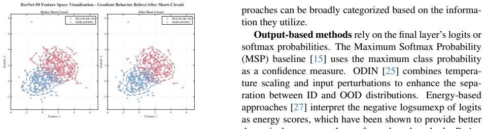
- [Figure 1] The caption does not state how the 2D projection is computed or which specific layer's embeddings are shown; please add a sentence describing the projection method and the layer used.
Circularity Check
The empirical OOD claim is benchmarked externally; only the Appendix A.1 'why it works' explanation is self-definitional.
-
self definitional
[Appendix A.1.1, Eq. (9)-(15) and Key Statement (A.1.1)]
"Sparsity Hypothesis for OOD. Suppose an OOD sample's high confidence stems from a small subset of coordinates in F. Formally, let I ⊂ {1, . . . , d} be such that [y]_c ≈ [y]_c | coords in I. That is, removing the dimensions in I would drastically reduce the logit [y]_c. ... Key Statement (A.1.1): For many OOD samples, most of the 'logit mass' is concentrated in a small set of coordinates."
The appendix presents this as the theoretical reason GSC is effective, but it assumes exactly the phenomenon to be explained. Eq. (9) defines I as the coordinates whose removal 'would drastically reduce the logit,' and Eq. (15) then derives that zeroing I reduces the logit by Σ_{i∈I} g_i F_i. This conclusion holds by definition of I, not from an independent property of the gradient. The only bridge from g to I is the assertion that the largest |g_i| values 'often identify' I, which is asserted rather than proven. Thus the explanatory chain reduces to the sparsity hypothesis; the empirical TopKRatio and benchmark results provide external support, but the formal 'why short-circuiting helps' argument is self-definitional.
full rationale
GSC's central quantitative claim is evaluated against external OOD benchmarks (CIFAR-10/100, ImageNet, Tiny-ImageNet), so the reported improvements are not manufactured from the method's own fitted constants. The 5% mask ratio and layer choice are tuned via ablations; no parameter is fitted to the test sets and then reported as a prediction. Algorithm 1's line 11 uses the full Jacobian (∇_F y)^T while line 6 only computes g = ∇_F [y]_c, which is a feasibility gap rather than a circularity. The identical baseline rows between Tables 2 and 3 and the text/table mismatches (e.g., 10.11% vs. 11.11% for iNaturalist) are correctness/reproducibility concerns, not circularity. The only circular element is the explanatory Appendix A.1, which restates the sparsity assumption as its key finding. Because that step is explanatory rather than the source of the benchmark numbers, the overall circularity score is low.
Assumptions & free parameters
free parameters (2)
- mask_ratio =
5%
- intervention_layer =
penultimate layer (final encoder output for ViTs)
assumptions (4)
- standard math The tail subnetwork f>L is Lipschitz-smooth near every feature vector, bounding the Taylor remainder by 0.5 L_smooth ||Delta F||^2.
- domain assumption OOD samples concentrate most of their logit gradient norm on a small set of feature coordinates.
- domain assumption ID samples have broad essential support with small per-coordinate logit share, so removing a few coordinates preserves most of the logit.
- ad hoc to paper The Fisher information matrix is diagonal with roughly equal lambda_i, so selecting by |g_i| approximates selecting by |g_i|/sqrt(lambda_i).
Cite this review
Pith. "Pith review of Gradient Short-Circuit: Efficient Out-of-Distribution Detection via Feature Intervention." pith.science (2026). https://pith.science/paper/UKVQJ3QM
@misc{pith2026250701417,
  author       = {Pith},
  title        = {Pith review of: Gradient Short-Circuit: Efficient Out-of-Distribution Detection via Feature Intervention},
  year         = {2026},
  howpublished = {\url{https://pith.science/paper/UKVQJ3QM}},
  note         = {Machine review of arXiv:2507.01417}
}
read the original abstract
Out-of-Distribution (OOD) detection is critical for safely deploying deep models in open-world environments, where inputs may lie outside the training distribution. During inference on a model trained exclusively with In-Distribution (ID) data, we observe a salient gradient phenomenon: around an ID sample, the local gradient directions for "enhancing" that sample's predicted class remain relatively consistent, whereas OOD samples--unseen in training--exhibit disorganized or conflicting gradient directions in the same neighborhood. Motivated by this observation, we propose an inference-stage technique to short-circuit those feature coordinates that spurious gradients exploit to inflate OOD confidence, while leaving ID classification largely intact. To circumvent the expense of recomputing the logits after this gradient short-circuit, we further introduce a local first-order approximation that accurately captures the post-modification outputs without a second forward pass. Experiments on standard OOD benchmarks show our approach yields substantial improvements. Moreover, the method is lightweight and requires minimal changes to the standard inference pipeline, offering a practical path toward robust OOD detection in real-world applications.
Figures


Figures from the paper (3 more)


Reference graph
Works this paper leans on
-
[1]
Line: Out-of-distribution detection by leveraging important neurons
Yong Hyun Ahn, Gyeong-Moon Park, and Seong Tae Kim. Line: Out-of-distribution detection by leveraging important neurons. In 2023 IEEE/CVF Conference on Computer Vi- sion and Pattern Recognition (CVPR), pages 19852–19862. IEEE, 2023. 1
work page 2023
-
[2]
Building nor- malizing flows with stochastic interpolants
Michael S Albergo and Eric Vanden-Eijnden. Building nor- malizing flows with stochastic interpolants. arXiv preprint arXiv:2209.15571, 2022
arXiv 2022
-
[3]
On the effectiveness of out-of-distribution data in self-supervised long-tail learning
Jianhong Bai, Zuozhu Liu, Hualiang Wang, Jin Hao, Yang Feng, Huanpeng Chu, and Haoji Hu. On the effectiveness of out-of-distribution data in self-supervised long-tail learning. arXiv preprint arXiv:2306.04934, 2023
arXiv 2023
-
[4]
Learning imbalanced datasets with label- distribution-aware margin loss
Kaidi Cao, Colin Wei, Adrien Gaidon, Nikos Arechiga, and Tengyu Ma. Learning imbalanced datasets with label- distribution-aware margin loss. Advances in neural informa- tion processing systems, 32, 2019
work page 2019
-
[5]
Adversarial reciprocal points learning for open set recognition
Guangyao Chen, Peixi Peng, Xiangqian Wang, and Yonghong Tian. Adversarial reciprocal points learning for open set recognition. IEEE Transactions on Pattern Analysis and Machine Intelligence, 44(11):8065–8081, 2021
work page 2021
-
[6]
Atom: Robustifying out-of-distribution detection using outlier mining
Jiefeng Chen, Yixuan Li, Xi Wu, Yingyu Liang, and Somesh Jha. Atom: Robustifying out-of-distribution detection using outlier mining. In Machine Learning and Knowledge Dis- covery in Databases. Research Track: European Conference, ECML PKDD 2021, Bilbao, Spain, September 13–17, 2021, Proceedings, Part III 21, pages 430–445. Springer, 2021. 1
work page 2021
-
[7]
Describing textures in the wild
Mircea Cimpoi, Subhransu Maji, Iasonas Kokkinos, Sammy Mohamed, and Andrea Vedaldi. Describing textures in the wild. In Proceedings of the IEEE conference on computer vision and pattern recognition, pages 3606–3613, 2014. 5
2014
-
[8]
Extremely simple activation shaping for out- of-distribution detection
Andrija Djurisic, Nebojsa Bozanic, Arjun Ashok, and Rosanne Liu. Extremely simple activation shaping for out- of-distribution detection. arXiv preprint arXiv:2209.09858,
Show all 55 references
-
[9]
An image is worth 16x16 words: Trans- formers for image recognition at scale
Alexey Dosovitskiy, Lucas Beyer, Alexander Kolesnikov, Dirk Weissenborn, Xiaohua Zhai, Thomas Unterthiner, Mostafa Dehghani, Matthias Minderer, Georg Heigold, Syl- vain Gelly, et al. An image is worth 16x16 words: Trans- formers for image recognition at scale. arXiv preprint a...
2010 arXiv
-
[10]
V os: Learning what you don’t know by virtual outlier synthesis
Xuefeng Du, Zhaoning Wang, Mu Cai, and Yixuan Li. V os: Learning what you don’t know by virtual outlier synthesis. arXiv preprint arXiv:2202.01197, 2022. 1
2022 arXiv
-
[11]
How does unlabeled data provably help out-of-distribution detection? arXiv preprint arXiv:2402.03502, 2024
Xuefeng Du, Zhen Fang, Ilias Diakonikolas, and Yixuan Li. How does unlabeled data provably help out-of-distribution detection? arXiv preprint arXiv:2402.03502, 2024. 1
2024 arXiv
-
[12]
Is out-of-distribution detection learnable? Advances in Neural Information Processing Systems , 35: 37199–37213, 2022
Zhen Fang, Yixuan Li, Jie Lu, Jiahua Dong, Bo Han, and Feng Liu. Is out-of-distribution detection learnable? Advances in Neural Information Processing Systems , 35: 37199–37213, 2022. 1
2022
-
[13]
Explaining and harnessing adversarial examples
Ian J Goodfellow, Jonathon Shlens, and Christian Szegedy. Explaining and harnessing adversarial examples. arXiv preprint arXiv:1412.6572, 2014. 2
2014 arXiv
-
[14]
Deep residual learning for image recognition
Kaiming He, Xiangyu Zhang, Shaoqing Ren, and Jian Sun. Deep residual learning for image recognition. In Proceed- ings of the IEEE conference on computer vision and pattern recognition, pages 770–778, 2016. 5
2016
-
[15]
A baseline for detect- ing misclassified and out-of-distribution examples in neural networks
Dan Hendrycks and Kevin Gimpel. A baseline for detect- ing misclassified and out-of-distribution examples in neural networks. arXiv preprint arXiv:1610.02136, 2016. 2, 5
2016 arXiv
-
[16]
Densely connected convolutional net- works
Gao Huang, Zhuang Liu, Laurens Van Der Maaten, and Kil- ian Q Weinberger. Densely connected convolutional net- works. In Proceedings of the IEEE conference on computer vision and pattern recognition, pages 4700–4708, 2017. 5
2017
-
[17]
On the impor- tance of gradients for detecting distributional shifts in the wild
Rui Huang, Andrew Geng, and Yixuan Li. On the impor- tance of gradients for detecting distributional shifts in the wild. Advances in Neural Information Processing Systems , 34:677–689, 2021. 2
2021
-
[19]
Galadrielle Humblot-Renaux, Sergio Escalera, and Thomas B Moeslund. A noisy elephant in the room: Is your out-of-distribution detector robust to label noise? In Proceedings of the IEEE/CVF Conference on Computer Vision and Pattern Recognition, pages 22626–22636, 2024. 1
2024
-
[20]
Learning multiple layers of features from tiny images
Alex Krizhevsky, Geoffrey Hinton, et al. Learning multiple layers of features from tiny images. 2009. 5
2009
-
[21]
Imagenet classification with deep convolutional neural net- works
Alex Krizhevsky, Ilya Sutskever, and Geoffrey E Hinton. Imagenet classification with deep convolutional neural net- works. Advances in neural information processing systems , 25, 2012. 5
2012
-
[22]
Simple and scalable predictive uncertainty estima- tion using deep ensembles
Balaji Lakshminarayanan, Alexander Pritzel, and Charles Blundell. Simple and scalable predictive uncertainty estima- tion using deep ensembles. Advances in neural information processing systems, 30, 2017. 3
2017
-
[23]
Tiny imagenet visual recognition challenge
Yann Le and Xuan Yang. Tiny imagenet visual recognition challenge. CS 231N, 7(7):3, 2015. 5
2015
-
[24]
A simple unified framework for detecting out-of-distribution samples and adversarial attacks
Kimin Lee, Kibok Lee, Honglak Lee, and Jinwoo Shin. A simple unified framework for detecting out-of-distribution samples and adversarial attacks. Advances in neural infor- mation processing systems, 31, 2018. 2, 5
2018
-
[25]
Enhanc- ing the reliability of out-of-distribution image detection in neural networks
Shiyu Liang, Yixuan Li, and Rayadurgam Srikant. Enhanc- ing the reliability of out-of-distribution image detection in neural networks. arXiv preprint arXiv:1706.02690, 2017. 2, 3, 5
2017 arXiv
-
[26]
Clustering with bregman divergences: an asymptotic analysis
Chaoyue Liu and Mikhail Belkin. Clustering with bregman divergences: an asymptotic analysis. Advances in neural in- formation processing systems, 29, 2016. 1
2016
-
[27]
Energy-based out-of-distribution detection
Weitang Liu, Xiaoyun Wang, John Owens, and Yixuan Li. Energy-based out-of-distribution detection. Advances in neural information processing systems, 33:21464–21475,
-
[28]
Towards deep learn- ing models resistant to adversarial attacks
Aleksander Madry, Aleksandar Makelov, Ludwig Schmidt, Dimitris Tsipras, and Adrian Vladu. Towards deep learn- ing models resistant to adversarial attacks. arXiv preprint arXiv:1706.06083, 2017. 2
2017 arXiv
-
[29]
Scanning trojaned models using out-of-distribution samples.Advances in Neural Information Processing Systems , 37:132545– 132582, 2025
Hossein Mirzaei, Ali Ansari, Bahar Dibaei Nia, Mojtaba Nafez, Moein Madadi, Sepehr Rezaee, Zeinab Taghavi, Arad Maleki, Kian Shamsaie, Mahdi Hajialilue, et al. Scanning trojaned models using out-of-distribution samples.Advances in Neural Information Processing Systems , 37:132...
2025
-
[30]
Importance estimation for neural net- work pruning
Pavlo Molchanov, Arun Mallya, Stephen Tyree, Iuri Fro- sio, and Jan Kautz. Importance estimation for neural net- work pruning. In Proceedings of the IEEE/CVF conference on computer vision and pattern recognition , pages 11264– 11272, 2019. 3
2019
-
[31]
Provable guarantees for un- derstanding out-of-distribution detection
Peyman Morteza and Yixuan Li. Provable guarantees for un- derstanding out-of-distribution detection. In Proceedings of the AAAI Conference on Artificial Intelligence, pages 7831– 7840, 2022. 2
2022
-
[32]
Gradients as features for deep representation learning
Fangzhou Mu, Yingyu Liang, and Yin Li. Gradients as features for deep representation learning. arXiv preprint arXiv:2004.05529, 2020. 2
2004 arXiv
-
[33]
Reading digits in natural images with unsupervised feature learning
Yuval Netzer, Tao Wang, Adam Coates, Alessandro Bis- sacco, Baolin Wu, Andrew Y Ng, et al. Reading digits in natural images with unsupervised feature learning. In NIPS workshop on deep learning and unsupervised feature learn- ing, page 4. Granada, 2011. 5
2011
-
[34]
Conjnorm: Tractable density estimation for out- of-distribution detection
Bo Peng, Yadan Luo, Yonggang Zhang, Yixuan Li, and Zhen Fang. Conjnorm: Tractable density estimation for out- of-distribution detection. arXiv preprint arXiv:2402.17888,
-
[35]
Ssd: A unified framework for self-supervised outlier detection
Vikash Sehwag, Mung Chiang, and Prateek Mittal. Ssd: A unified framework for self-supervised outlier detection. arXiv preprint arXiv:2103.12051, 2021. 2
2021 arXiv
-
[36]
Dice: Leveraging sparsification for out-of-distribution detection
Yiyou Sun and Yixuan Li. Dice: Leveraging sparsification for out-of-distribution detection. In European conference on computer vision, pages 691–708. Springer, 2022. 2
2022
-
[37]
React: Out-of- distribution detection with rectified activations
Yiyou Sun, Chuan Guo, and Yixuan Li. React: Out-of- distribution detection with rectified activations. Advances in neural information processing systems , 34:144–157, 2021. 2, 3, 5
2021
-
[38]
Out- of-distribution detection with deep nearest neighbors
Yiyou Sun, Yifei Ming, Xiaojin Zhu, and Yixuan Li. Out- of-distribution detection with deep nearest neighbors. In In- ternational Conference on Machine Learning, pages 20827– 20840. PMLR, 2022. 2, 3, 5
2022
-
[39]
Pure: Prompt evolution with graph ode for out-of-distribution fluid dynamics mod- eling
Hao Wu, Changhu Wang, Fan Xu, Jinbao Xue, Chong Chen, Xian-Sheng Hua, and Xiao Luo. Pure: Prompt evolution with graph ode for out-of-distribution fluid dynamics mod- eling. Advances in Neural Information Processing Systems, 37:104965–104994, 2025. 1
2025
-
[40]
Sun database: Large-scale scene recognition from abbey to zoo
Jianxiong Xiao, James Hays, Krista A Ehinger, Aude Oliva, and Antonio Torralba. Sun database: Large-scale scene recognition from abbey to zoo. In 2010 IEEE computer so- ciety conference on computer vision and pattern recognition, pages 3485–3492. IEEE, 2010. 5
2010
-
[41]
Turkergaze: Crowdsourcing saliency with webcam based eye tracking
Pingmei Xu, Krista A Ehinger, Yinda Zhang, Adam Finkel- stein, Sanjeev R Kulkarni, and Jianxiong Xiao. Turkergaze: Crowdsourcing saliency with webcam based eye tracking. arXiv preprint arXiv:1504.06755, 2015. 5
2015 arXiv
-
[42]
Generalized out-of-distribution detection: A survey
Jingkang Yang, Kaiyang Zhou, Yixuan Li, and Ziwei Liu. Generalized out-of-distribution detection: A survey. Inter- national Journal of Computer Vision , 132(12):5635–5662,
-
[43]
Lsun: Construction of a large-scale image dataset using deep learning with humans in the loop
Fisher Yu, Ari Seff, Yinda Zhang, Shuran Song, Thomas Funkhouser, and Jianxiong Xiao. Lsun: Construction of a large-scale image dataset using deep learning with humans in the loop. arXiv preprint arXiv:1506.03365, 2015. 5
2015 arXiv
-
[44]
logit mass
Bolei Zhou, Agata Lapedriza, Aditya Khosla, Aude Oliva, and Antonio Torralba. Places: A 10 million image database for scene recognition. IEEE transactions on pattern analysis and machine intelligence, 40(6):1452–1464, 2017. 5 A. Theoretical Analysis Overview In this appendix, ...
2017
-
[45]
Forward x 7→ F 7→ y: cost Ω(Forward>L)
-
[46]
Backward y 7→ g: compute g = ∇F [y]c, cost Ω(Backward>L)
-
[47]
Hence the total is Ω(Forward>L) + Ω(Backward >L) + O(d)
Local Approx: y′ approx ≈ y + ( ∇Fy)⊤(F′ − F), cost O(d). Hence the total is Ω(Forward>L) + Ω(Backward >L) + O(d). In many networks, Ω(Forward>L) ≈ Ω(Backward>L). Compared to the naive ap- proach 2 Ω(Forward>L), we reduce overhead by roughly half, ignoring the relatively minor...
-
[48]
Accuracy: We exploit OOD samples’ fragile re- liance on a small subset of coordinates, gener- ating a minimal perturbation ∆F that collapses OOD confidence
-
[49]
parameter-like
Efficiency: We skip a second forward pass through f>L, approximating y′ via a lightweight dot product. As a result, our combined strategy excels in both accuracy (major OOD suppression) and efficiency (time-saving at inference). Empirical results con- firm this synergy in prac...
-
[50]
, λd) with λi > 0
I(F) is diagonal and satisfies I(F) = diag(λ1, . . . , λd) with λi > 0
-
[51]
The budget constraint is ∆F⊤ I(F) ∆F ≤ κ
-
[52]
Then the solution that minimizes L(F + ∆F) subject to the Fisher constraint is given bynulli- fying or scaling the top-k coordinates of F with largest |gi|/√λi
We consider small perturbations ∥∆F∥ so that L(F + ∆F) ≈ L(F) + g⊤∆F. Then the solution that minimizes L(F + ∆F) subject to the Fisher constraint is given bynulli- fying or scaling the top-k coordinates of F with largest |gi|/√λi. In particular, Gradient Short- Circuit impleme...
-
[53]
Fisher Metric: The Fisher information matrix I(F) captures local model sensitivity
-
[54]
Fisher distance
Constraint Geometry: Limiting ∆F⊤ I(F) ∆F corresponds to small “Fisher distance” moves from F
-
[55]
Optimality: Under diagonal or near-diagonal Fisher assumptions, short-circuiting largest- gradient coordinates is the optimal local solution to minimize OOD confidence. This viewpoint unifies Gradient Short-Circuit with a second-order information geometry, reinforcing that GSC...
-
[100]
Block2 + Penultimate
Each approach uses a 5% mask ratio (top gradient coordi- nates for GSC, smallest gradient for Reverse, random selection for Random). We display averaged FPR95 (%) and AUROC (%) across six OOD sets. Mask Strategy FPR95 (%) ↓ AUROC (%)↑ Random 45.32 88.73 Reverse 62.18 83.42 GSC...
Reviewed August 6, 2026 · model on record in the stance chip above.
Discussion (0). Continue with ORCID to comment.