REVIEW 5 major objections 5 minor 87 references
Large-scale portfolio optimization with variational neural annealing
T0 review · 5 major / 5 minor · reviewed 2026-08-06 · deepseek-v4-flash
Pith's one-line read The paper claims that variational neural annealing solves mixed-integer nonlinear portfolio optimization on universes of more than 2,000 assets, with solution quality comparable to a leading commercial solver and faster convergence on…
desk verdict A legitimate new application of VNA to portfolio optimization, with a solid Mosek benchmark on solution quality; but the advertised speed advantage and universal-scaling claims don't survive close reading. read the letter →
The pith
A machine-rendered reading of the paper's core claim, the machinery that carries it, and where it could break.
The reading
What carries the argument
The load-bearing object is the variational neural annealing algorithm. It uses a recurrent neural network as an autoregressive ansatz, $P_\theta(x) = \prod_i P_\theta(x_i | x_{i-1}, \ldots, x_1)$, and trains it at each temperature to minimize the variational free energy $F_\theta = \langle H\rangle_\theta + T \sum_x P_\theta(x) \ln P_\theta(x)$, so that $P_\theta$ approaches the Boltzmann distribution $e^{-H/T}$. The temperature follows a geometric schedule from large $T$ to zero, and at the end the network generates uncorrelated candidate portfolios that are filtered for constraint satisfaction. The RNN gives $O(N)$ cost per gradient step and is what lets the method scale past 2,000 assets; for the finite-size scaling study the normalization constraint is enforced with both a penalty and a Lagrange-multiplier term.
What would settle it
A decisive check would be to extend the same dynamical finite-size scaling to a fourth index or to synthetic portfolios of intermediate size with many more trading months; if the rescaled data do not collapse onto one curve, or if the fitted exponents drift with the chosen set of sizes, the claimed universality and $N^{0.58}$ annealing-time scaling are refuted. In parallel, letting Mosek run to its standard 0.01% gap on the Russell 3000 instance and comparing Sharpe ratios month by month would test the competitiveness claim directly.
Extended reading notes
Core claim
The central claim is that VNA, in its classical recurrent-neural-network form, solves the mixed-integer nonlinear portfolio optimization problem at real-world index scale. The authors encode the Markowitz objective with normalization, transaction-cost, turnover, and volatility constraints as a Hamiltonian $H(x)$ with penalty and Lagrange-multiplier terms, turning each asset's weight into a discrete decision variable. VNA minimizes the variational free energy $F_\theta = \langle H\rangle_\theta + T \sum_x P_\theta(x) \ln P_\theta(x)$ along a geometric annealing schedule, using an autoregressive RNN whose per-gradient-step cost is $O(N)$. On the S&P 500 the residual energy decays as a power law, $e_{\mathrm{rel}} \propto \tau_a^{-1.43(1)}$; on the Russell 3000, VNA reaches Sharpe ratios close to Mosek's, with a reported time-to-solution of 2,580 seconds versus 6,709 seconds for Mosek (which had its gap tolerance relaxed to 1% because the standard 0.01% threshold was not reached in days). Treating the three indices as increasing system sizes and five trading months as disorder realizations, the authors obtain a data collapse of $e_{\mathrm{rel}} N^{\kappa}$ against $\tau_a N^{\mu}$ with $\mu = -0.58 \pm 0.08$ and $\kappa = 0.16 \pm 0.09$, which they interpret as universal critical dynamics and polynomial annealing-time scaling.
Load-bearing premise
The load-bearing premise is that the S&P 500, Russell 1000, and Russell 3000 behave like three sizes of the same optimization problem, and that five trading months are enough trading periods to stand in for many random instances; if that premise fails, the universal scaling curve and its exponents are a fitting artifact.
Editorial extensions
If this is right
- Portfolio optimization with transaction costs, turnover limits, and volatility caps can be treated as a generic Hamiltonian minimization, so the same VNA pipeline applies without requiring convexity or differentiability.
- Near-optimal portfolios for universes of more than 2,000 assets are within reach of variational methods, and on hard instances VNA can reach comparable Sharpe ratios in less wall-clock time than a commercial solver.
- The extracted exponents imply that the annealing steps needed for near-adiabatic performance grow roughly as $N^{0.58}$, a polynomial cost in the number of assets.
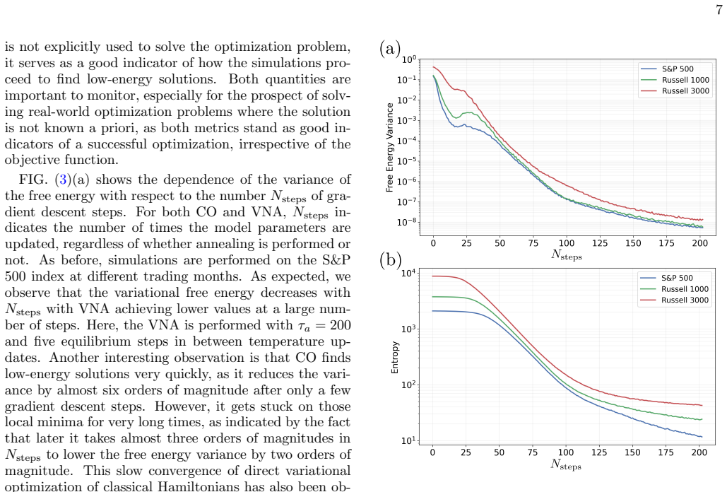
- Physics-inspired diagnostics such as free-energy variance and Von Neumann entropy can serve as proxies for solution quality when the optimum is unknown.
- Constraint feasibility, not energy minimization, becomes the practical bottleneck: on Russell 3000 the fraction of valid samples can fall to 0.129% for some months, so penalty and Lagrange-multiplier tuning is decisive.
Reading between the lines
- The Ising-style encoding is asset-agnostic, so the same pipeline should transfer to bond portfolios, multi-asset funds, or crypto baskets with discrete position sizes; the paper tests equities only.
- The scaling collapse implies an out-of-sample forecast: a hypothetical 4,000-asset index should land on the same collapsed curve, so its residual energy could be predicted from the spline without solving the optimization; running that forecast would be a sharp test of universality.
- The validity failures on Russell 3000 suggest that penalty tuning, not the neural sampler, is the main barrier to production use; an adaptive augmented-Lagrangian update scheme, which the authors list as future work, would be the natural remedy.
Editorial analysis
A structured set of objections, weighed in public.
Referee Report
Summary. The paper proposes Variational Neural Annealing (VNA) with recurrent neural networks as a classical solver for a mixed-integer nonlinear portfolio-optimization problem. The objective is written as an Ising-like Hamiltonian with penalty terms for normalization, transaction costs, volatility, and turnover. The authors report that VNA scales to more than 2,000 assets, compares favorably with Mosek in Sharpe ratio, and exhibits power-law decay of relative energy with annealing steps. They further perform a dynamical finite-size scaling analysis over the S&P 500, Russell 1000, and Russell 3000, reporting a data collapse with exponents mu = -0.58 +/- 0.08 and kappa = 0.16 +/- 0.09, and a polynomial annealing-time scaling. The paper concludes that VNA is a practical large-scale MINLP solver and that the scaling behavior is universal.
Significance. If the central claims were fully supported, the work would be a useful contribution connecting statistical-physics-inspired methods to practical large-scale portfolio optimization. The paper has genuine strengths: the Sharpe-ratio comparison against Mosek in Figures 6-7 is an external benchmark, the annealing-vs-direct-optimization ablation in Figures 3-4 is internally consistent, the use of real index data is appropriate for the application, and the authors are candid about limitations such as low feasibility rates in Appendix C. However, the headline universal-scaling claim is not established by the evidence presented: the three indices are not independent realizations of one optimization ensemble, the collapse uses only three system sizes, and the reduced Hamiltonian of Eq. (14) differs from the full MINLP benchmarked earlier. Because the abstract's two central claims are performance comparability and universal scaling, the scaling weakness is load-bearing.
major comments (5)
- [Section IV E, Eq. (15), Fig. 8, Appendix D] The DFSS universal-scaling claim is not supported by the presented evidence. The three 'system sizes' are the S&P 500, Russell 1000, and Russell 3000, which are nested or heavily overlapping universes with different composition, factor structure, and constraint activity, not independent realizations of a single optimization ensemble. With only three system sizes, the two-parameter collapse e_rel = N^{-kappa} g(tau_a N^mu) is flexible enough to fit three smooth curves, and the bootstrap errors in Appendix D reflect only within-index month-to-month noise, not the dominant uncertainty from using non-identical ensembles. An out-of-sample test, such as leave-one-index-out prediction or the use of genuinely independent asset universes, is needed before universal behavior and polynomial annealing-time scaling can be claimed.
- [Section IV B, Eq. (13)] The relative energy e_rel is normalized by E_ref, which is the lowest objective value found by VNA itself at tau_a = 1000, or in Fig. 2(b) by the lowest value over N_units. Thus e_rel measures closeness to VNA's own best solution, not closeness to an external or true optimum. The exponents extracted in Fig. 8 may therefore characterize VNA's internal convergence rather than solution quality relative to the global optimum. For at least one system size, E_ref should be cross-checked against an independent solver such as Mosek on the same reduced objective, or the interpretation of the scaling exponents should be restricted accordingly.
- [Section IV E, Eq. (14) vs Section IV D, Table I] The DFSS analysis is performed on a reduced Hamiltonian that includes only the normalization constraint, explicitly relaxing the full constraint set used in the Mosek benchmark. The abstract and conclusions use this analysis to support VNA's scalability on the full MINLP, but the connection is not established. Either the DFSS analysis should be repeated on the full constraint set, or the scalability claim should be explicitly limited to the reduced problem defined by Eq. (14).
- [Section IV D, Table I] The time-to-solution comparison in Table I is not apples-to-apples. VNA times are fixed wall-clock runtimes on four NVIDIA A100 GPUs, whereas Mosek times are times to reach a relative MIP gap of 0.01%, or 1% for Russell 3000, on 64 CPU threads; the hardware, stopping rules, and post-hoc sample filtering differ. The text calls the comparison 'qualitative,' but the abstract states that VNA exhibits 'faster convergence on hard instances' without presenting controlled solution-quality-versus-time curves. Please provide per-method quality-versus-time comparisons or a same-budget comparison, or soften the claimed speed advantage.
- [Section IV D and Appendix C] The claim that VNA can identify near-optimal solutions for portfolios of more than 2,000 assets is qualified by the fact that valid solutions were not obtained for all trading months in Fig. 7, and Appendix C reports Russell 3000 feasibility as low as 0.129%. The fraction of months without valid solutions and the sensitivity to penalty coefficients should be stated in the main text, since they directly affect the headline practical claim.
minor comments (5)
- [Throughout] Several section headings contain unintended spaces, such as 'POR TFOLIO OPTIMIZA TION FORMULA TION', 'T ransaction Costs', and 'V ersus'; these should be corrected.
- [Section IV B, Eq. (13)] The definition of E_ref differs between Fig. 2(a) and Fig. 2(b), but the text does not clearly distinguish the two definitions; please state the reference value used in each panel.
- [Section IV E, Eq. (15)] The statement that the annealing time scales as tau_a ~ N^{-mu} is confusing because mu is negative; writing the positive exponent tau_a ~ N^{0.58} would make the polynomial growth explicit.
- [Appendix A, Fig. 9] The fit range for the power-law exponent -1.43(1) is described as 'over the last number of annealing steps'; please specify the exact fit range and the number of points used.
- [Section IV E, Fig. 8 caption] The caption says each data point is averaged over five independent trading months, but it is not stated whether the same five months are used for all three indices; if they differ, the collapse is even less controlled and the caption should say so.
Circularity Check
No significant circularity: VNA is benchmarked externally against Mosek, and the DFSS exponents are openly fitted rather than derived.
full rationale
The paper's primary performance claim does not reduce to its own inputs: VNA solutions are benchmarked against the commercial solver Mosek on Sharpe ratio and time-to-solution (Section IV D, Figs. 6 and 7, Table I), so 'near-optimal' and 'comparable to state-of-the-art optimizers' are judged against an external solver, not against VNA's own best run. The dynamical finite-size scaling analysis (Section IV E, Eq. (15)) estimates exponents kappa, mu and a spline g by minimizing a residual cost on the same e_rel data (Appendix D, Eq. (D4)); this is an in-sample fit, and the paper transparently says the exponents are 'extracted from this collapse' and gives bootstrap uncertainties. Fitting a scaling collapse and then displaying the collapsed curves is standard practice, not a circular derivation: the exponents are not assumed in the definition of e_rel, and the collapse could in principle fail. The limitations the paper itself acknowledges, including the small number of system sizes, the use of only five trading months as disorder averages, and the absence of an out-of-sample forecast test, are statistical validity concerns about overfitting and ensemble comparability, not cases where a prediction is equivalent to its input by construction. Section IV E explicitly notes 'a limited number of data points' and uncertainties in the exponents, and Appendix C reports that VNA 'did not yield valid solutions for all trading months'; these are honest caveats weighing on correctness, not circularity. The self-citation to the VNA algorithm [57] supplies the method, but the portfolio results are validated independently against Mosek, so the citation is not load-bearing in a circular sense. No equation in the paper reduces an output to a fitted parameter or to a self-citation chain.
Assumptions & free parameters
free parameters (8)
- Risk aversion coefficient ρ_v
- Normalization penalty ρ_n
- Fixed-cost penalty ρ_c
- Volatility bound V and penalty coefficient
- Turnover bound T and penalty coefficient ρ_t
- Transaction cost coefficients γ_v and γ_f
- Lagrange multiplier λ_n
- Algorithm hyperparameters (N_units, τ_a, learning rate, schedule, sample size)
assumptions (6)
- domain assumption Markowitz mean-variance objective with historical mean returns and covariance is a valid model for portfolio choice.
- domain assumption An autoregressive RNN can approximate the Boltzmann distribution of the portfolio Hamiltonian sufficiently well.
- domain assumption Minimizing variational free energy at each annealing step guides the samples to the ground state at zero temperature.
- domain assumption Finite penalty coefficients plus post-hoc filtering yield feasible solutions.
- ad hoc to paper Different indices and trading months behave like different system sizes and disorder realizations of the same optimization ensemble.
- domain assumption Historical returns remain stationary across the five-year lookback and the trading months tested.
Cite this review
Pith. "Pith review of Large-scale portfolio optimization with variational neural annealing." pith.science (2026). https://pith.science/paper/P7WAEPMZ
@misc{pith2026250707159,
  author       = {Pith},
  title        = {Pith review of: Large-scale portfolio optimization with variational neural annealing},
  year         = {2026},
  howpublished = {\url{https://pith.science/paper/P7WAEPMZ}},
  note         = {Machine review of arXiv:2507.07159}
}
read the original abstract
Portfolio optimization is a routine asset management operation conducted in financial institutions around the world. However, under real-world constraints such as turnover limits and transaction costs, its formulation becomes a mixed-integer nonlinear program that current mixed-integer optimizers often struggle to solve. We propose mapping this problem onto a classical Ising-like Hamiltonian and solving it with Variational Neural Annealing (VNA), via its classical formulation implemented using autoregressive neural networks. We demonstrate that VNA can identify near-optimal solutions for portfolios comprising more than 2,000 assets and yields performance comparable to that of state-of-the-art optimizers, such as Mosek, while exhibiting faster convergence on hard instances. Finally, we present a dynamical finite-size scaling analysis applied to the S&P 500, Russell 1000, and Russell 3000 indices, revealing universal behavior and polynomial annealing time scaling of the VNA algorithm on portfolio optimization problems.
Figures


Figures from the paper (9 more)



Reference graph
Works this paper leans on
-
[1]
Structure and binding of Lennard–Jones clusters: 13≤N≤147,
J. A. Northby, “Structure and binding of Lennard–Jones clusters: 13≤N≤147,” The Journal of Chemical Physics87, 6166–6177 (1987)
1987
-
[2]
Thermodynamics and the global optimization of Lennard-Jones clusters,
Jonathan P. K. Doye, David J. Wales, and Mark A. Miller, “Thermodynamics and the global optimization of Lennard-Jones clusters,” The Journal of Chemical Physics109, 8143–8153 (1998)
1998
-
[3]
9 (World Scien- tific Publishing Company, 1987)
Marc M´ ezard, Giorgio Parisi, and Miguel Angel Vira- soro,Spin glass theory and beyond: an introduction to the replica method and its applications, Vol. 9 (World Scien- tific Publishing Company, 1987)
1987
-
[4]
Spin glasses: a computational challenge for the 21st century,
A. P. Young, “Spin glasses: a computational challenge for the 21st century,” Computer Physics Communications 146, 107–112 (2002)
2002
-
[5]
Optimization in computational systems biology,
Julio R. Banga, “Optimization in computational systems biology,” BMC Systems Biology2, 47 (2008)
2008
-
[6]
Optimization algorithms for computational systems bi- ology,
Federico Reali, Corrado Priami, and Luca Marchetti, “Optimization algorithms for computational systems bi- ology,” Frontiers in Applied Mathematics and Statistics 3, 6 (2017)
2017
-
[7]
Application of combinatorial optimization strategies in synthetic biol- ogy,
Gita Naseri and Mattheos A. G. Koffas, “Application of combinatorial optimization strategies in synthetic biol- ogy,” Nature Communications11, 2446 (2020)
work page 2020
-
[8]
Healthcare scheduling in optimization context: a re- view,
Zahraa A. Abdalkareem, Amiza Amir, Mohammed Azmi Al-Betar, Phaklen Ekhan, and Abdelaziz I. Hammouri, “Healthcare scheduling in optimization context: a re- view,” Health and Technology11, 445–469 (2021)
work page 2021
Show all 87 references
-
[9]
The flexible job shop scheduling problem: A review,
“The flexible job shop scheduling problem: A review,” 14 European Journal of Operational Research314, 409–432 (2024)
2024
-
[10]
A survey of job shop scheduling problem: The types and models,
Hegen Xiong, Shuangyuan Shi, Danni Ren, and Jinjin Hu, “A survey of job shop scheduling problem: The types and models,” Computers & Operations Research142, 105731 (2022)
2022
-
[11]
Portfolio selection,
Harry Markowitz, “Portfolio selection,” The Journal of Finance7, 77–91 (1952)
1952
-
[12]
On the computational complexity of Ising spin glass models,
Francisco Barahona, “On the computational complexity of Ising spin glass models,” Journal of Physics A: Math- ematical and General15, 3241 (1982)
1982
-
[13]
Ising formulations of many NP prob- lems,
Andrew Lucas, “Ising formulations of many NP prob- lems,” Frontiers in physics2, 5 (2014)
2014
-
[14]
Mixed- integer nonlinear optimization,
Pietro Belotti, Christian Kirches, Sven Leyffer, Jeff Lin- deroth, James Luedtke, and Ashutosh Mahajan, “Mixed- integer nonlinear optimization,” Acta Numerica22, 1– 131 (2013)
2013
-
[15]
Solvable model of a spin-glass,
David Sherrington and Scott Kirkpatrick, “Solvable model of a spin-glass,” Physical Review Letters35, 1792 (1975)
1975
-
[16]
Rational decisions, random matrices and spin glasses,
Stefano Galluccio, Jean-Philippe Bouchaud, and Marc Potters, “Rational decisions, random matrices and spin glasses,” Physica A: Statistical Mechanics and its Appli- cations259, 449–456 (1998)
1998
-
[17]
Tax-aware portfolio construction via convex optimization,
Nicholas Moehle, Mykel J. Kochenderfer, Stephen Boyd, and Andrew Ang, “Tax-aware portfolio construction via convex optimization,” Journal of Optimization Theory and Applications189, 364–383 (2021)
2021
-
[18]
Quantum computing for finance: overview and prospects,
Rom´ an Or´ us, Samuel Mugel, and Enrique Lizaso, “Quantum computing for finance: overview and prospects,” Reviews in Physics4, 100028 (2019)
2019
-
[19]
Quan- tum computing for finance: state-of-the-art and future prospects,
Daniel J Egger, Claudio Gambella, Jakub Marecek, Scott McFaddin, Martin Mevissen, Rudy Raymond, Andrea Si- monetto, Stefan Woerner, and Elena Yndurain, “Quan- tum computing for finance: state-of-the-art and future prospects,” IEEE Transactions on Quantum Engineering 1, 1–24 (2020)
2020
-
[20]
Quantum computing for finance,
Dylan Herman, Cody Googin, Xiaoyuan Liu, Yue Sun, Alexey Galda, Ilya Safro, Marco Pistoia, and Yuri Alex- eev, “Quantum computing for finance,” Nature Reviews Physics5, 450–465 (2023)
2023
-
[21]
Quantum compu- tational finance: quantum algorithm for portfolio opti- mization,
Patrick Rebentrost and Seth Lloyd, “Quantum compu- tational finance: quantum algorithm for portfolio opti- mization,” KI-K¨ unstliche Intelligenz , 1–12 (2024)
2024
-
[22]
From portfolio optimization to quantum blockchain and security: A systematic review of quan- tum computing in finance,
Abha Satyavan Naik, Esra Yeniaras, Gerhard Hellstern, Grishma Prasad, and Sanjay Kumar Lalta Prasad Vishwakarma, “From portfolio optimization to quantum blockchain and security: A systematic review of quan- tum computing in finance,” Financial Innovation11, 1– 67 (2025)
2025
-
[23]
Quantum annealing with manufactured spins,
Mark W. Johnson, Mohammad H. S. Amin, Suzanne Gildert, Trevor Lanting, Firas Hamze, Neil Dickson, Richard Harris, Andrew J. Berkley, Jan Johansson, Paul Bunyk,et al., “Quantum annealing with manufactured spins,” Nature473, 194–198 (2011)
2011
-
[24]
Solving the optimal trading trajectory problem using a quantum annealer,
Gili Rosenberg, Poya Haghnegahdar, Phil Goddard, Pe- ter Carr, Kesheng Wu, and Marcos L´ opez De Prado, “Solving the optimal trading trajectory problem using a quantum annealer,” inProceedings of the 8th workshop on high performance computational finance(2015) pp. 1–7
2015
-
[25]
Reverse quantum annealing approach to portfolio optimization problems,
Davide Venturelli and Alexei Kondratyev, “Reverse quantum annealing approach to portfolio optimization problems,” Quantum Machine Intelligence1, 17–30 (2019)
2019
-
[26]
Dynamic portfolio optimiza- tion with real datasets using quantum processors and quantum-inspired tensor networks,
Samuel Mugel, Carlos Kuchkovsky, Escol´ astico S´ anchez, Samuel Fern´ andez-Lorenzo, Jorge Luis-Hita, Enrique Lizaso, and Rom´ an Or´ us, “Dynamic portfolio optimiza- tion with real datasets using quantum processors and quantum-inspired tensor networks,” Physical Review Re- s...
2022
-
[27]
Quantum portfolio optimization with investment bands and target volatil- ity,
Samuel Palmer, Serkan Sahin, Rodrigo Hernandez, Samuel Mugel, and Roman Orus, “Quantum portfolio optimization with investment bands and target volatil- ity,” arXiv preprint arXiv:2106.06735 (2021)
2021 arXiv
-
[28]
Quantum walk-based portfolio optimi- sation,
Nicholas Slate, Edric Matwiejew, Samuel Marsh, and Jingbo B Wang, “Quantum walk-based portfolio optimi- sation,” Quantum5, 513 (2021)
2021
-
[29]
Bench- marking the performance of portfolio optimization with QAOA,
Sebastian Brandhofer, Daniel Braun, Vanessa Dehn, Ger- hard Hellstern, Matthias H¨ uls, Yanjun Ji, Ilia Polian, Amandeep Singh Bhatia, and Thomas Wellens, “Bench- marking the performance of portfolio optimization with QAOA,” Quantum Information Processing22, 25 (2022)
2022
-
[30]
Wasser- stein solution quality and the Quantum Approximate Optimization Algorithm: a portfolio optimization case study,
Jack S. Baker and Santosh Kumar Radha, “Wasser- stein solution quality and the Quantum Approximate Optimization Algorithm: a portfolio optimization case study,” arXiv preprint arXiv:2202.06782 (2022)
2022 arXiv
-
[31]
Best practices for portfolio optimization by quantum comput- ing, experimented on real quantum devices,
Giuseppe Buonaiuto, Francesco Gargiulo, Giuseppe De Pietro, Massimo Esposito, and Marco Pota, “Best practices for portfolio optimization by quantum comput- ing, experimented on real quantum devices,” Scientific Reports13, 19434 (2023)
2023
-
[32]
A quantum approximate optimization algorithm,
Edward Farhi, Jeffrey Goldstone, and Sam Gutmann, “A quantum approximate optimization algorithm,” arXiv preprint arXiv:1411.4028 (2014)
2014 arXiv
-
[33]
A variational eigenvalue solver on a photonic quantum processor,
Alberto Peruzzo, Jarrod McClean, Peter Shadbolt, Man- Hong Yung, Xiao-Qi Zhou, Peter J Love, Al´ an Aspuru- Guzik, and Jeremy L O’brien, “A variational eigenvalue solver on a photonic quantum processor,” Nature com- munications5, 4213 (2014)
2014
-
[34]
A review on Quantum Approximate Optimization Algorithm and its variants,
Kostas Blekos, Dean Brand, Andrea Ceschini, Chiao-Hui Chou, Rui-Hao Li, Komal Pandya, and Alessandro Sum- mer, “A review on Quantum Approximate Optimization Algorithm and its variants,” Physics Reports1068, 1–66 (2024)
2024
-
[35]
Challenges and opportuni- ties in quantum optimization,
Amira Abbas, Andris Ambainis, Brandon Augustino, Andreas B¨ artschi, Harry Buhrman, Carleton Coffrin, Giorgio Cortiana, Vedran Dunjko, Daniel J Egger, Bruce G Elmegreen,et al., “Challenges and opportuni- ties in quantum optimization,” Nature Reviews Physics , 1–18 (2024)
2024
-
[36]
Branch-and-bound digitized counterdiabatic quantum optimization,
Anton Simen, Sebasti´ an V Romero, Alejandro Gomez Cadavid, Enrique Solano, and Narendra N Hegade, “Branch-and-bound digitized counterdiabatic quantum optimization,” arXiv preprint arXiv:2504.15367 (2025)
2025 arXiv
-
[37]
The density-matrix renormalization group in the age of matrix product states,
Ulrich Schollw¨ ock, “The density-matrix renormalization group in the age of matrix product states,” Annals of physics326, 96–192 (2011)
2011
-
[38]
and has far-reaching implications [69–72]. However, SA gives an exact solution only in the limit of an in- finitely slow annealing schedule; for any finite annealing schedule, the solution diverges significantly as SA fails to exactly sample the equilibrium Boltzmann distribu-...
2008
-
[39]
Optimization by simulated annealing,
Scott Kirkpatrick, C Daniel Gelatt Jr, and Mario P Vec- chi, “Optimization by simulated annealing,” Science220, 671–680 (1983)
1983
-
[40]
Strategic portfolio optimization using simulated, digital, and quantum annealing,
Jonas Lang, Sebastian Zielinski, and Sebastian Feld, “Strategic portfolio optimization using simulated, digital, and quantum annealing,” Applied Sciences12(2022), 10.3390/app122312288
2022 doi
-
[41]
Ising-model optimizer with parallel-trial bit-sieve engine,
Satoshi Matsubara, Hirotaka Tamura, Motomu Takatsu, Danny Yoo, Behraz Vatankhahghadim, Hironobu Ya- masaki, Toshiyuki Miyazawa, Sanroku Tsukamoto, Ya- 15 suhiro Watanabe, Kazuya Takemoto,et al., “Ising-model optimizer with parallel-trial bit-sieve engine,” inCom- plex, Intelli...
2017
-
[42]
Physics-inspired optimization for quadratic unconstrained problems using a digital annealer,
Maliheh Aramon, Gili Rosenberg, Elisabetta Valiante, Toshiyuki Miyazawa, Hirotaka Tamura, and Helmut G. Katzgraber, “Physics-inspired optimization for quadratic unconstrained problems using a digital annealer,” Fron- tiers in Physics7, 48 (2019)
2019
-
[43]
Solving the optimal trading trajectory problem using simulated bifurcation,
Kyle Steinhauer, Takahisa Fukadai, and Sho Yoshida, “Solving the optimal trading trajectory problem using simulated bifurcation,” arXiv preprint arXiv:2009.08412 (2020)
2020 arXiv
-
[44]
Real-time trad- ing system based on selections of potentially profitable, uncorrelated, and balanced stocks by NP-hard combi- natorial optimization,
Kosuke Tatsumura, Ryo Hidaka, Jun Nakayama, Tomoya Kashimata, and Masaya Yamasaki, “Real-time trad- ing system based on selections of potentially profitable, uncorrelated, and balanced stocks by NP-hard combi- natorial optimization,” IEEE Access11, 120023–120033 (2023)
2023
-
[45]
Enhancing combinatorial optimization with classical and quantum generative models,
Javier Alcazar, Mohammad Ghazi Vakili, Can B. Kalayci, and Alejandro Perdomo-Ortiz, “Enhancing combinatorial optimization with classical and quantum generative models,” Nature Communications15, 2761 (2024)
2024
-
[46]
Deep learning for portfolio optimization,
Zihao Zhang, Stefan Zohren, and Stephen Roberts, “Deep learning for portfolio optimization,” The Journal of Financial Data Science2, 8–20 (2020)
2020
-
[47]
Enhancing Markowitz’s portfolio selection paradigm with machine learning,
Marcos L´ opez de Prado, Joseph Simonian, Francesco A. Fabozzi, and Frank J. Fabozzi, “Enhancing Markowitz’s portfolio selection paradigm with machine learning,” An- nals of Operations Research (2024), 10.1007/s10479-024- 06257-1
2024 doi
-
[48]
Deep learning in finance: a survey of applications and tech- niques,
Ebikella Mienye, Nobert Jere, George Obaido, Ibo- moiye Domor Mienye, and Kehinde Aruleba, “Deep learning in finance: a survey of applications and tech- niques,” AI5, 2066–2091 (2024)
2024
-
[49]
Large Language Models in finance: a survey,
Yinheng Li, Shaofei Wang, Han Ding, and Hang Chen, “Large Language Models in finance: a survey,” (2024), arXiv:2311.10723
2024 arXiv
-
[50]
Neural networks for portfo- lio analysis with cardinality constraints,
Xinwei Cao and Shuai Li, “Neural networks for portfo- lio analysis with cardinality constraints,” IEEE Trans- actions on Neural Networks and Learning Systems35, 17674–17687 (2024)
2024
-
[51]
Deep reinforcement learning for opti- mal portfolio allocation: a comparative study with mean- variance optimization,
Srijan Sood, Kassiani Papasotiriou, Marius Vaiciulis, and Tucker Balch, “Deep reinforcement learning for opti- mal portfolio allocation: a comparative study with mean- variance optimization,” inProceedings of the Interna- tional Conference on Automated Planning and Schedul- in...
2023
-
[52]
FreQuant: a reinforcement-learning based adaptive portfolio optimization with multi-frequency decomposi- tion,
Jihyeong Jeon, Jiwon Park, Chanhee Park, and U Kang, “FreQuant: a reinforcement-learning based adaptive portfolio optimization with multi-frequency decomposi- tion,” inProceedings of the 30th ACM SIGKDD Confer- ence on Knowledge Discovery and Data Mining, KDD ’24 (Association ...
2024
-
[53]
Graph neural networks for deep portfolio optimization,
¨Omer Ekmekcio˘ glu and Mustafa C ¸ . Pınar, “Graph neural networks for deep portfolio optimization,” Neural Com- puting and Applications35, 20663–20674 (2023)
2023
-
[54]
StockGPT: a GenAI model for stock predic- tion and trading,
Dat Mai, “StockGPT: a GenAI model for stock predic- tion and trading,” (2024), arXiv:2404.05101
2024 arXiv
-
[55]
E2EAI: End-to- End deep learning framework for active investing,
Zikai Wei, Bo Dai, and Dahua Lin, “E2EAI: End-to- End deep learning framework for active investing,” in Proceedings of the Fourth ACM International Conference on AI in Finance, ICAIF ’23 (Association for Computing Machinery, New York, NY, USA, 2023) pp. 55–63
2023
-
[56]
Advancing in- vestment frontiers: industry-grade deep reinforce- ment learning for portfolio optimization,
Philip Ndikum and Serge Ndikum, “Advancing in- vestment frontiers: industry-grade deep reinforce- ment learning for portfolio optimization,” (2024), arXiv:2403.07916
2024 arXiv
-
[57]
End- to-end risk budgeting portfolio optimization with neural networks,
A. Sinem Uysal, Xiaoyue Li, and John M. Mulvey, “End- to-end risk budgeting portfolio optimization with neural networks,” Annals of Operations Research339, 397–426 (2024)
2024
-
[58]
Variational neural annealing,
Mohamed Hibat-Allah, Estelle M. Inack, Roeland Wiersema, Roger G. Melko, and Juan Carrasquilla, “Variational neural annealing,” Nature Machine Intelli- gence3, 952–961 (2021)
2021
-
[59]
Lattice protein folding with varia- tional annealing,
Shoummo Ahsan Khandoker, Estelle M. Inack, and Mo- hamed Hibat-Allah, “Lattice protein folding with varia- tional annealing,” (2025), arXiv:2502.20632
2025 arXiv
-
[60]
From deep learning to LLMs: a survey of AI in quantitative invest- ment,
Bokai Cao, Saizhuo Wang, Xinyi Lin, Xiaojun Wu, Hao- han Zhang, Lionel M. Ni, and Jian Guo, “From deep learning to LLMs: a survey of AI in quantitative invest- ment,” (2025), arXiv:2503.21422
2025 arXiv
-
[61]
MILLION: a general multi-objective framework with controllable risk for portfolio management,
Liwei Deng, Tianfu Wang, Yan Zhao, and Kai Zheng, “MILLION: a general multi-objective framework with controllable risk for portfolio management,” (2024), arXiv:2412.03038
2024 arXiv
-
[62]
Sparse autoregressive neural networks for classical spin sys- tems,
Indaco Biazzo, Dian Wu, and Giuseppe Carleo, “Sparse autoregressive neural networks for classical spin sys- tems,” Machine Learning: Science and Technology5, 025074 (2024)
2024
-
[63]
Message passing variational autoregressive network for solving intractable Ising models,
Qunlong Ma, Zhi Ma, Jinlong Xu, Hairui Zhang, and Ming Gao, “Message passing variational autoregressive network for solving intractable Ising models,” Communi- cations Physics7, 236 (2024)
2024
-
[64]
Efficient opti- mization of variational autoregressive networks with nat- ural gradient,
Jing Liu, Ying Tang, and Pan Zhang, “Efficient opti- mization of variational autoregressive networks with nat- ural gradient,” Physical Review E111, 025304 (2025)
2025
-
[65]
Supplementing recurrent neural networks with annealing to solve combinatorial optimization problems,
Shoummo Ahsan Khandoker, Jawaril Munshad Abedin, and Mohamed Hibat-Allah, “Supplementing recurrent neural networks with annealing to solve combinatorial optimization problems,” Machine Learning: Science and Technology4, 015026 (2023)
2023
-
[66]
Investigating topological order using recurrent neural networks,
Mohamed Hibat-Allah, Roger G. Melko, and Juan Car- rasquilla, “Investigating topological order using recurrent neural networks,” Physical Review B108, 075152 (2023)
2023
-
[67]
Recurrent neu- ral network wave functions for rydberg atom arrays on kagome lattice,
Mohamed Hibat-Allah, Ejaaz Merali, Giacomo Torlai, Roger G. Melko, and Juan Carrasquilla, “Recurrent neu- ral network wave functions for rydberg atom arrays on kagome lattice,” (2024), arXiv:2405.20384
2024 arXiv
-
[68]
Leverag- ing recurrence in neural network wavefunctions for large- scale simulations of heisenberg antiferromagnets: the tri- angular lattice,
M. Schuyler Moss, Roeland Wiersema, Mohamed Hibat- Allah, Juan Carrasquilla, and Roger G. Melko, “Leverag- ing recurrence in neural network wavefunctions for large- scale simulations of heisenberg antiferromagnets: the tri- angular lattice,” (2025), arXiv:2505.20406
2025
-
[69]
Mosek optimization suite,
MOSEK ApS, “Mosek optimization suite,”https:// www.mosek.com
-
[70]
A Survey of simulated annealing applications to operations research problems,
C. Koulamas, S.R. Antony, and R. Jaen, “A Survey of simulated annealing applications to operations research problems,” Omega22, 41–56 (1994)
1994
-
[71]
A tutorial survey of theory and applica- tions of simulated annealing,
Bruce Hajek, “A tutorial survey of theory and applica- tions of simulated annealing,” in1985 24th IEEE Con- ference on Decision and Control(1985) pp. 755–760. 16
1985
-
[72]
Optimization by simulated an- nealing: an experimental evaluation; Part II, graph color- ing and number partitioning,
David S. Johnson, Cecilia R. Aragon, Lyle A. McGeoch, and Catherine Schevon, “Optimization by simulated an- nealing: an experimental evaluation; Part II, graph color- ing and number partitioning,” Operations Research39, 378–406 (1991)
1991
-
[73]
Robust design of multimachine power sys- tem stabilizers using simulated annealing,
M. A. Abido, “Robust design of multimachine power sys- tem stabilizers using simulated annealing,” IEEE Trans- actions on Energy Conversion15, 297–304 (2000)
2000
-
[74]
Recur- rent neural network wave functions,
Mohamed Hibat-Allah, Martin Ganahl, Lauren E. Hay- ward, Roger G. Melko, and Juan Carrasquilla, “Recur- rent neural network wave functions,” Physical Review Research2, 023358 (2020)
2020
-
[75]
Iterative retraining of quantum spin models using recurrent neural networks,
Christopher Roth, “Iterative retraining of quantum spin models using recurrent neural networks,” (2020), arXiv:2003.06228
2020 arXiv
-
[76]
Quantum critical dynamics in a 5,000-qubit pro- grammable spin glass,
Andrew D King, Jack Raymond, Trevor Lanting, Richard Harris, Alex Zucca, Fabio Altomare, Andrew J Berkley, Kelly Boothby, Sara Ejtemaee, Colin Enderud,et al., “Quantum critical dynamics in a 5,000-qubit pro- grammable spin glass,” Nature617, 61–66 (2023)
2023
-
[77]
Pushing the boundary of quantum advantage in hard combinato- rial optimization with probabilistic computers,
Shuvro Chowdhury, Navid Anjum Aadit, Andrea Grimaldi, Eleonora Raimondo, Atharva Raut, P. Aaron Lott, Johan H. Mentink, Marek M. Rams, Federico Ricci-Tersenghi, Massimo Chiappini, Luke S. Theog- arajan, Tathagata Srimani, Giovanni Finocchio, Ma- soud Mohseni, and Kerem Y. Cams...
2025
-
[78]
Ibm ilog cplex optimizer,
IBM ILOG, “Ibm ilog cplex optimizer,”https://www. ibm.com/products/ilog-cplex-optimization-studio
-
[79]
Gurobi optimizer,
Gurobi Optimization, LLC, “Gurobi optimizer,”http: //www.gurobi.com
-
[80]
Uni- versal nonequilibrium quantum dynamics in imaginary time,
C. De Grandi, A. Polkovnikov, and A. W. Sandvik, “Uni- versal nonequilibrium quantum dynamics in imaginary time,” Phys. Rev. B84, 224303 (2011)
2011
-
[81]
Scaling ad- vantage in approximate optimization with quantum an- nealing,
Humberto Munoz-Bauza and Daniel Lidar, “Scaling ad- vantage in approximate optimization with quantum an- nealing,” Phys. Rev. Lett.134, 160601 (2025)
2025
-
[82]
Nonlinear programming,
Dimitri P Bertsekas, “Nonlinear programming,” Journal of the Operational Research Society48, 334–334 (1997)
1997
-
[83]
Wright,Numerical Opti- mization, 2nd ed., Springer Series in Operations Research and Financial Engineering (Springer New York, NY, New York, NY, 2006) pp
Jorge Nocedal and Stephen J. Wright,Numerical Opti- mization, 2nd ed., Springer Series in Operations Research and Financial Engineering (Springer New York, NY, New York, NY, 2006) pp. XXII+664
2006
-
[84]
Dynamic scaling at classical phase transitions approached through nonequilibrium quenching,
Cheng-Wei Liu, Anatoli Polkovnikov, and Anders W. Sandvik, “Dynamic scaling at classical phase transitions approached through nonequilibrium quenching,” Phys. Rev. B89, 054307 (2014)
2014
-
[85]
Learning con- strained optimization with deep augmented lagrangian methods,
James Kotary and Ferdinando Fioretto, “Learning con- strained optimization with deep augmented lagrangian methods,” (2024), arXiv:2403.03454
2024 arXiv
-
[86]
An adaptive augmented lagrangian method for training physics and equality constrained artificial neural networks,
Shamsulhaq Basir and Inanc Senocak, “An adaptive augmented lagrangian method for training physics and equality constrained artificial neural networks,” (2023), arXiv:2306.04904
2023 arXiv
-
[87]
A mea- sure of data collapse for scaling,
Somendra M Bhattacharjee and Flavio Seno, “A mea- sure of data collapse for scaling,” Journal of Physics A: Mathematical and General34, 6375–6380 (2001)
2001
Reviewed August 6, 2026 · model on record in the stance chip above.
Discussion (0). Sign in to comment.