Goal-Oriented Sequential Bayesian Experimental Design for Causal Learning

Jiayuan Dong; Jie Liu; Xun Huan (University of Michigan); Zheyu Zhang

REVIEW 3 major objections 5 minor 76 references

Goal-Oriented Sequential Bayesian Experimental Design for Causal Learning

T0 review · 3 major / 5 minor · reviewed 2026-08-06 · deepseek-v4-flash

Challenge this review Re-run · record.json Download PDF Read on arXiv ↗

Pith's one-line read GO-CBED argues that sequential causal experiments should target a user-specified causal query rather than the whole model, and shows such goal-oriented planning beats full-model and myopic baselines in tested settings.

desk verdict A sound combination of known BOED pieces with credible causal-discovery results; the causal-reasoning headline is provisional because the evaluation metric is the same variational bound the policy optimizes. read the letter →

arxiv 2507.07359 v1 pith:AHRXXBRF submitted 2025-07-10 cs.LG cs.AIstat.MEstat.ML

Zheyu Zhang , Jiayuan Dong , Jie Liu , Xun Huan (University of Michigan) This is my paper

classification cs.LGcs.AIstat.MEstat.ML

keywords causalexperimentaldesignBayesianoptimalgoal-orientedexpectedinformationgainnon-myopicplanningamortizedpolicylearningnormalizingflowsgeneregulatorynetworks

verification ladder T0 review T1 audit T2 compute T3 formal

The pith

A machine-rendered reading of the paper's core claim, the machinery that carries it, and where it could break.

The reading

This paper tries to establish that sequential causal experiments should be goal-oriented: when what you want is the answer to a specific causal question — say, the effect of intervening on one gene on another — the interventions you run should be chosen to reduce uncertainty about that query, not to reconstruct the whole causal model. The proposed framework, GO-CBED, treats experiment selection as a planning problem and learns an amortized policy that maximizes the expected information gain about the query over an entire sequence of interventions, rather than greedily one experiment at a time. Because the exact information gain is intractable, the paper optimizes a variational lower bound, training the policy and the variational posterior jointly. Across synthetic structural causal models and semi-synthetic gene regulatory networks, the paper reports that GO-CBED consistently outperforms baselines that learn the full model or pick interventions greedily, with the largest gains under limited experimental budgets and nonlinear causal mechanisms. A sympathetic reader would care because experiments are expensive, and the gap between 'good for the model' and 'good for the question' is exactly the gap this framework attacks.

What carries the argument

The load-bearing pieces are: (1) the query-expected information gain of Eq. (4), $I_T(\pi)$, defined through the posterior predictive $p(z|h_T)$ of the user-specified causal quantity $z=H(M;\epsilon_z)$ (an interventional effect such as $X_i^{do(X_j=\psi_j)}$, or the graph $G$ itself); (2) the variational lower bound of Theorem 4.1, $I_{T;L}(\pi;\lambda,\phi) \le I_T(\pi)$, obtained by substituting a learned posterior density $q_\lambda(z|f_\phi(h_T))$ for the intractable $p(z|h_T)$, so that optimization reduces to maximizing the log-density of that approximation; (3) a transformer policy network with alternating attention over variables and history, permutation-invariant across history samples and permutation-equivariant across variables, with a Gumbel-softmax head for discrete intervention targets; and (4) normalizing-flow posteriors (a stack of invertible coupling layers) for causal-effect queries and independent-Bernoulli per-edge posteriors for graph queries. The training loop draws models and queries from the prior, simulates intervention trajectories, and updates policy, embedding, and variational parameters together by gradient ascent on the lower bound, producing an amortized policy whose deployment cost is a single forward pass.

What would settle it

Take a structural-uncertainty setting from Section 5.2 and compute the true expected information gain for GO-CBED and each baseline using a high-accuracy estimator such as nested Monte Carlo with very large inner-loop sizes. If GO-CBED's variational lower bound exceeds the baselines' while its estimated true expected information gain is equal or lower, the paper's central claim of consistent superiority in causal reasoning would be contradicted on that setting.

Watch

Extended reading notes

Core claim

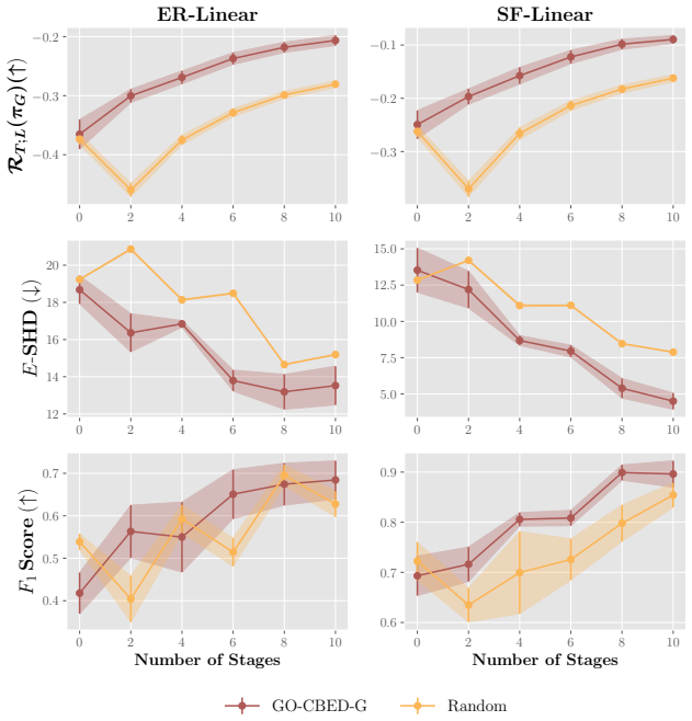
The central claim is that the right objective for causal experimental design is the expected information gain on the causal quantity of interest, $I_T(\pi) = \mathbb{E}_{p(M)p(h_T|M,\pi)p(z|M)}[\log p(z|h_T)/p(z)]$, and that a policy maximizing this query-specific objective outperforms policies that maximize information about the full model, about the graph structure alone, or that choose each intervention greedily. The paper shows that when the query $z$ is not a bijective function of the model $M$, targeting the query directly is more efficient because no experimental effort is spent on model aspects irrelevant to the query. To make the objective tractable, the paper proves a variational lower bound $I_{T;L}(\pi;\lambda,\phi) \le I_T(\pi)$, tight when the learned posterior matches the true posterior, and maximizes it jointly over a transformer-based policy network and flexible variational posteriors (normalizing flows for causal-effect queries, per-edge Bernoulli factors for graph queries). Empirically, the paper claims GO-CBED consistently achieves higher query EIG than full-model, structure-learning, myopic, and random baselines on synthetic and semi-synthetic tasks, with the advantage growing for nonlinear mechanisms and short experimental budgets.

Load-bearing premise

The causal-reasoning comparisons are measured with the same variational lower bound the proposed method is trained to maximize; if that bound is looser for the proposed method's chosen trajectories than for the baselines', the reported performance gap could overstate the true information gain.

Editorial extensions

If this is right

When causal queries are the goal, experiments designed for the query extract more information per intervention than experiments designed for the full model; the paper's fixed-graph example shows a parameter-trained policy performs substantially worse on the query than a query-trained policy.
In nonlinear and biologically structured settings, a policy trained for causal discovery can underperform even random intervention selection for query-specific inference, meaning an accurate graph is not a reliable proxy for good query uncertainty reduction.
Non-myopic planning pays off over time: the reported advantage over greedy and random baselines grows after the early stages, so the framework's value increases with longer experiment sequences.
Deployment is real-time: because the policy is amortized, intervention selection at experiment time costs a single forward pass with cost independent of sequence length, with no online Bayesian inference required.
The approach is most valuable under exactly the conditions the paper argues typify biological research: limited experimental budgets and complex, nonlinear causal mechanisms.

Reading between the lines

Editorial extensions of the paper, not claims the author makes directly.

A direct test the paper does not run would estimate the true expected information gain under structural uncertainty with a high-accuracy estimator and compare GO-CBED to baselines on that quantity, since the causal-reasoning results are scored on the variational lower bound GO-CBED itself maximizes; if that bound is easier to fit on GO-CBED's trajectories than on the baselines', the reported gap c
Because the policy is trained against a prior over graphs and mechanisms, a misspecified prior will be inherited by the query-optimal policy; a perturbation study over priors would clarify how much of the reported gain survives real-world prior uncertainty, a question the paper's own limitations section leaves open.
Extending the objective to heterogeneous experimental costs would likely widen the advantage of goal-oriented design, since the paper's motivation is that experiments are expensive but costs enter only implicitly through the fixed budget.
The observation that some nodes are equally informative for structure and for the query (where the discovery and query policies perform similarly) points to an open theoretical question: characterize when query-optimal and structure-learning designs coincide.

Share X Bluesky LinkedIn Reddit HN

Editorial analysis

A structured set of objections, weighed in public.

Desk editor's note, referee report, and a circularity audit.

Desk Editor's Note

read the letter

Quick take: this is a well-built synthesis of existing ideas, and the causal-discovery experiments are genuinely informative. The causal-reasoning claims, which are the distinctive contribution, should be read with caution until the bound gap is checked under structural uncertainty.

What's actually new: a non-myopic, amortized policy for goal-oriented causal experimental design, trained by maximizing a variational lower bound on EIG for a user-specified causal query. The pieces—variational bounds, normalizing-flow posteriors, transformer policies, RL training—are all known, but the specific combination targeting causal queries rather than full-model learning is a real step beyond Toth et al.'s myopic ABCI and the structure-only non-myopic methods. The math in Theorem 4.1 and Proposition A.1 is standard and correct. The experiments are extensive: synthetic ER/SF graphs, linear and nonlinear mechanisms, DREAM-based gene regulatory networks, and discovery metrics (E-SHD, F1) that are grounded in ground truth. I also appreciate that they train dedicated posterior networks per policy to reduce confounding when comparing policies.

The soft spot is load-bearing. In Sections 5.2 and D.2, the causal-reasoning results report R_{T;L}(π), the same variational lower bound that GO-CBED jointly optimizes in Eq. (6). Theorem 4.1 only tells you it's a lower bound; it doesn't control the gap under structural uncertainty. A policy can inflate the bound by choosing trajectories where the amortized flow posterior is easier to fit, without increasing true EIG. Figure 8 validates posterior tightness only in the fixed-graph, linear-Gaussian setting. Under structural uncertainty, p(z|h_T) is a mixture over graphs and is typically multimodal; no diagnostic shows the flow posterior fits equally well for GO-CBED-z versus GO-CBED-G or Random. So the headline "GO-CBED outperforms on causal reasoning" may partly reflect posterior fit rather than information gain. The NMC comparison in Section 5.1 is also confounded by NMC's downward bias at small inner-loop sizes, which the paper itself notes. And ABCI, the closest goal-oriented policy, is never benchmarked as a policy; that is a notable omission for positioning.

That said, these are not fatal. The discovery results in Section 5.3 using E-SHD and F1 are much less affected, and the framework itself is sound. If the authors add a bound-gap diagnostic under structural uncertainty and benchmark ABCI, I'd be fairly convinced. No code or data is released, which limits reproducibility despite a detailed appendix.

Who this is for: researchers in Bayesian experimental design or active causal discovery who care about targeted queries and sequential planning. It deserves a serious referee. I'd send it to review, with the bound-gap issue as the main requested revision.

Referee Report

3 major / 5 minor

Summary. GO-CBED proposes a non-myopic, goal-oriented framework for sequential Bayesian experimental design in causal systems. The target causal query z is fixed by the user, and the method maximizes a variational lower bound on the expected information gain for z, jointly optimizing a transformer-based policy network and a variational posterior (normalizing flows for causal reasoning, product-Bernoulli for causal discovery). The paper presents a theoretical lower-bound result, a fixed-graph motivating example, causal reasoning experiments on synthetic and DREAM-derived networks, and causal discovery experiments evaluated with EIG lower bound, expected structural Hamming distance, and F1 score.

Significance. If the reported results hold, the paper makes a useful step beyond full-model and myopic causal BOED: it provides an amortized, non-myopic policy that targets user-specified causal queries, and the discovery experiments use ground-truth structural metrics that give credible evidence for structure recovery. The variational derivation in Theorem 4.1 is correct, and the paper is transparent about some limitations. The central causal-reasoning claim, however, is currently supported only by comparisons on the same variational lower bound that GO-CBED optimizes, and the closest goal-oriented myopic baseline is not benchmarked, so the distinctive claims are not yet established at the level promised in the abstract.

major comments (3)

[Section 5.2, Eqs. (5)-(6), Theorem 4.1] The causal-reasoning evaluation uses RT;L(pi;lambda,phi), the same variational lower bound that GO-CBED jointly maximizes in Eq. (6). From Theorem 4.1, RT;L is RT minus the expected KL divergence between the true posterior p(z|hT) and the variational q_lambda(z|f_phi(hT)). A policy can therefore increase RT;L by selecting trajectories on which q_lambda is easier to fit, even if true EIG is unchanged or lower. The paper validates posterior tightness only in the fixed-graph linear-Gaussian setting of Figure 8; under structural uncertainty, p(z|hT) is a mixture over graphs and parameters and is generally multimodal. The reported gains of GO-CBED-z over GO-CBED-G and Random in Figures 3, 4, and 13 could partly reflect different approximation gaps rather than different true information gain. This issue is load-bearing for the goal-oriented causal-reasoning claims. Please provide a per-policy comparison against an unbiased estimate of true EIG (for example, large-sample NMC or exact computation where available) under structural uncertainty, or report diagnostics that the bound gap is comparable across policies.
[Section 5.2, Figures 3-4 and 13] The paper motivates GO-CBED against myopic goal-oriented design, citing Toth et al. [63] as the closest prior work, but the causal-reasoning experiments compare only GO-CBED-z, GO-CBED-G, and Random. Without the myopic goal-oriented baseline, the empirical claim that non-myopic goal-oriented planning outperforms existing goal-oriented methods is not supported. Please add a comparison with the Toth et al. method (or an equivalent myopic goal-oriented baseline) in the causal-reasoning experiments, or substantially temper the corresponding claims in the abstract and introduction.
[Section 5.1 and Appendix D.1] The NMC baseline comparison is confounded as a policy comparison because the NMC estimator with finite inner-loop samples is downward biased, as the paper itself notes in Appendix D.1, while the GO-CBED curves report a variational lower bound. Although the direction of the comparison may be conservative for GO-CBED, it does not provide a clean measurement of which policy achieves higher true EIG, especially since the GO-CBED panel in Figure 2 uses RT;L for its own policies. Using a common evaluation metric across all policies, such as a large-sample NMC estimate or exact EIG in the linear-Gaussian example, would make the comparison unambiguous.

minor comments (5)

[Appendix A.4, Eq. (A10)] There is a typo: 'Lt the transformation' should be 'Let the transformation'; the notation for the Jacobian determinant terms could also be cleaned up for readability.
[Appendix D.1, Figure 12] The legend label 'GO-OED' is inconsistent with the name 'GO-CBED' used throughout the rest of the paper; please standardize the label.
[Appendix C.3.2] The query definitions for the four panels of Figure 3 are listed without explicitly mapping each query to its panel; please make that mapping clear in the text or table.
[Section 4.2, Eq. (7)] The product-Bernoulli posterior is defined over all i,j edge indicators without an explicit acyclicity constraint, while the true graph posterior is supported only on DAGs; please clarify how cyclic graphs are excluded in training and evaluation, including any renormalization.
[General] The paper does not state whether code and trained models will be released; a reproducibility statement would be helpful, especially since the method is amortized and the hyperparameters are reported in the appendix.

Circularity Check

1 steps flagged · score 6.0 of 10

The causal-reasoning comparisons are scored on R_{T;L}, the same variational lower bound that GO-CBED-z is explicitly trained to maximize, so part of the reported EIG advantage is by construction and the bound gap under structural uncertainty is never controlled.

fitted input called prediction [Eq. (6) in Section 4.1; Section 5.2; Figures 3, 4, 13; Appendix A.2 proof of Theorem 4.1]
"π∗, λ∗, ϕ∗ ∈ arg max_{π,λ,ϕ} [ R_{T ;L}(π; λ, ϕ) := E_{p(M)p(h_T |M,π)p(z|M)}[ log q_λ(z|f_ϕ(h_T)) ] ] ... Figure 3: Performance comparison of policies trained for T = 10 on causal queries ... R_{T ;L}(π_z)(↑) ... I_T(π) − I_{T ; L}(π; λ, ϕ) = E_{p(h_T |π)}[ D_KL( p(z|h_T ) || q_λ(z|f_ϕ(h_T )) ) ]"

GO-CBED-z selects π, λ, and φ jointly to maximize R_{T;L} in Eq. (6), and the causal-reasoning results in Figures 3, 4, and 13 report R_{T;L}(π_z) as the headline metric. The proof of Theorem 4.1 shows R_T(π) − R_{T;L}(π; λ, φ) = E[ D_KL(p(z|h_T) || q_λ(z|f_φ(h_T))) ], so the reported quantity can be increased by choosing trajectories on which the amortized normalizing-flow posterior is easier to fit, without increasing the true EIG R_T. The paper checks posterior tightness only in the fixed-graph setting (Figure 8); under structural uncertainty p(z|h_T) is a multimodal mixture and no bound-gap diagnostic is provided for GO-CBED-z versus GO-CBED-G or Random.

full rationale

The variational lower bound itself is derived self-containedly: Theorem 4.1 is proved in Appendix A.2 from the non-negativity of the KL divergence, with no load-bearing self-citation. The causal-discovery experiments in Section 5.3 additionally report ground-truth E-SHD and F1 metrics computed from simulated SCMs and DREAM subnetworks, so those claims have independent support. The circularity is confined to, but load-bearing for, the goal-oriented causal-reasoning claims: R_{T;L} is simultaneously the objective optimized in Eq. (6) for GO-CBED-z and the evaluation metric in the causal-reasoning figures, and the variational gap is not quantified under structural uncertainty. This makes part of the reported EIG advantage reduce by construction to the training objective, though not to full definitional equivalence: Theorem 4.1 is a genuine inequality, and the fixed-graph tightness check in Figure 8 provides partial supporting evidence. The NMC baseline comparison in Section 5.1 is also confounded by NMC's downward bias at small inner-loop sizes, which the paper itself acknowledges; this is a benchmarking weakness rather than an additional circular step.

Assumptions & free parameters 5 free parameters · 4 assumptions · 0 invented entities

The theory is standard variational BOED mathematics and requires no fitted scientific constants. The empirical pipeline introduces numerous hand-chosen hyperparameters (architecture sizes, temperatures, learning rates, flow-layer counts) and simulation priors (graph priors, noise variances, neural-network weight priors) that the reported gains depend on, but none enter the analytical derivations in Theorem 4.1 or Proposition A.1. The main non-standard assumption is that the variational posteriors are flexible enough to make lower-bound comparisons meaningful across policies, which is checked only in one fixed-graph example. No new physical entities are introduced.

free parameters (5)

Gumbel-softmax temperature schedule tau = min(5 * 0.9995^step, 0.1)
Hand-chosen annealing schedule for discrete intervention target selection; affects training stability and exploration but not the theoretical bound.
Number of RealNVP coupling layers n_trans = 4
Hand-chosen flexibility of the normalizing-flow posterior for causal reasoning queries; larger values could change bound tightness and empirical results.
Posterior edge logit bias and temperature initializations = Bias -3, Temp 2
Initial values for learnable parameters in the Bernoulli graph posterior; chosen by hand and affecting causal discovery posterior quality.
Learning rates and scheduler = 5e-4/1e-4 with ExponentialLR gamma=0.8
Hand-chosen optimization hyperparameters for policy and posterior networks; affect convergence and reported performance.
Training batch size n_env and steps n_step = 10 environments per step; 10000-15000 steps
Computational budget choices; larger budgets could change the quality of the trained policy and variational posterior.

assumptions (4)

domain assumption Causal sufficiency and independent exogenous noise for interventional Markov factorization
Invoked in Eq. (2): 'Assuming causal sufficiency and independent noise [56], the interventional distribution follows the Markov factorization'. This is load-bearing for the likelihood used in training and EIG estimation.
domain assumption Availability of a prior over graph structures and mechanisms
The policy is trained by sampling M = (G, theta) from the prior, and the authors state in the Limitations that GO-CBED's effectiveness depends on the availability of prior knowledge over causal structures and mechanisms.
ad hoc to paper The variational families (RealNVP flows and product-Bernoulli graph posteriors) are flexible enough to make the lower bound tight or the bound gap comparable across policies
Theorem 4.1 gives tightness only in the limit; the comparisons in Sections 5.1 and 5.2 assume the bound gap is small or similar across policies, validated only in the fixed-graph example (Figure 8).
standard math Standard information-theoretic identities: chain rule of mutual information and data-processing inequality
Used in Proposition A.1 (telescoping sum for incremental EIG) and in the argument that a non-invertible query z makes targeted design more efficient than full-model design.

how reviews work

0 comments

Cite this review

Pith. "Pith review of Goal-Oriented Sequential Bayesian Experimental Design for Causal Learning." pith.science (2026). https://pith.science/paper/AHRXXBRF

@misc{pith2026250707359,
  author       = {Pith},
  title        = {Pith review of: Goal-Oriented Sequential Bayesian Experimental Design for Causal Learning},
  year         = {2026},
  howpublished = {\url{https://pith.science/paper/AHRXXBRF}},
  note         = {Machine review of arXiv:2507.07359}
}

read the original abstract

We present GO-CBED, a goal-oriented Bayesian framework for sequential causal experimental design. Unlike conventional approaches that select interventions aimed at inferring the full causal model, GO-CBED directly maximizes the expected information gain (EIG) on user-specified causal quantities of interest, enabling more targeted and efficient experimentation. The framework is both non-myopic, optimizing over entire intervention sequences, and goal-oriented, targeting only model aspects relevant to the causal query. To address the intractability of exact EIG computation, we introduce a variational lower bound estimator, optimized jointly through a transformer-based policy network and normalizing flow-based variational posteriors. The resulting policy enables real-time decision-making via an amortized network. We demonstrate that GO-CBED consistently outperforms existing baselines across various causal reasoning and discovery tasks-including synthetic structural causal models and semi-synthetic gene regulatory networks-particularly in settings with limited experimental budgets and complex causal mechanisms. Our results highlight the benefits of aligning experimental design objectives with specific research goals and of forward-looking sequential planning.

Figures

Figures reproduced from arXiv: 2507.07359 by the authors.

**Figure 2.** Performance comparison of policies trained for [PITH_FULL_IMAGE:figures/full_fig_p006_2.png] view at source ↗

**Figure 3.** Performance comparison of policies trained for [PITH_FULL_IMAGE:figures/full_fig_p007_3.png] view at source ↗

Figures from the paper (17 more)

**Figure 4.** Figure 4: Performance comparison of policies trained for T = 10 on E. coli gene regulatory networks with nonlinear causal mechanisms (d = 10). GO-CBED-z performs comparably to baselines in early stages but exhibits rapid improvement after stage 3, ultimately achieving substanti…

**Figure 5.** Figure 5: Performance comparison on synthetic SCMs, using ER and SF graph priors with linear and [PITH_FULL_IMAGE:figures/full_fig_p008_5.png]

**Figure 6.** Figure 6: GO-CBED outperforms all baselines on semi-synthetic [PITH_FULL_IMAGE:figures/full_fig_p009_6.png]

**Figure 7.** Figure 7: Policy network architecture. The model takes as input a three-dimensional tensor of [PITH_FULL_IMAGE:figures/full_fig_p019_7.png]

**Figure 8.** Figure 8: Comparison between the true posterior predictive distribution [PITH_FULL_IMAGE:figures/full_fig_p021_8.png]

**Figure 9.** Figure 9: Evaluation of policies on ER and SF graphs with both linear and nonlinear causal mech [PITH_FULL_IMAGE:figures/full_fig_p022_9.png]

**Figure 10.** Figure 10: Evaluation of policies on E. coli graphs with nonlinear causal mechanisms. The π ∗ G demonstrates strong performance in accurately identifying the underlying causal graph. available, the posterior is instantiated via substitution as qλ(fϕ(D∗ )). Samples from this dist…

**Figure 11.** Figure 11: Evaluation of interventions on node 1 using integers from [PITH_FULL_IMAGE:figures/full_fig_p024_11.png]

**Figure 12.** Figure 12: Prior-omitted EIG lower bound estimates, with parenthesis values denoting the inner loop [PITH_FULL_IMAGE:figures/full_fig_p024_12.png]

**Figure 13.** Figure 13: Additional causal reasoning experiments on nonlinear gene regulatory networks. [PITH_FULL_IMAGE:figures/full_fig_p025_13.png]

**Figure 14.** Figure 14: Performance comparison on synthetic SCMs, with each method using its originally [PITH_FULL_IMAGE:figures/full_fig_p026_14.png]

**Figure 15.** Figure 15: Performance comparison on semi-synthetic gene regulatory ( [PITH_FULL_IMAGE:figures/full_fig_p026_15.png]

**Figure 16.** Figure 16: Causal discovery performance on nonlinear [PITH_FULL_IMAGE:figures/full_fig_p027_16.png]

**Figure 17.** Figure 17: Causal discovery performance on linear Yeast gene regulatory networks. GO-CBED [PITH_FULL_IMAGE:figures/full_fig_p027_17.png]

**Figure 18.** Figure 18: Causal discovery performance on nonlinear Yeast gene regulatory networks. GO-CBED [PITH_FULL_IMAGE:figures/full_fig_p027_18.png]

**Figure 19.** Figure 19: Evaluation of GO-CBED under a distributional shift in observation noise at deployment [PITH_FULL_IMAGE:figures/full_fig_p028_19.png]

**Figure 20.** Figure 20: Evaluation of GO-CBED under a distributional shift in observation noise at deployment [PITH_FULL_IMAGE:figures/full_fig_p029_20.png]

Discussion (0). Sign in to comment.

Reference graph

Works this paper leans on

76 extracted references · 69 canonical work pages

[63]

Toth, C., Lorch, L., Knoll, C., Krause, A., Pernkopf, F., Peharz, R., and V on Kügelgen, J. (2022). Active Bayesian causal inference. Advances in Neural Information Processing Systems, 35:16261–16275

work page 2022
[1]

Agrawal, R., Squires, C., Yang, K., Shanmugam, K., and Uhler, C. (2019). Abcd-strategy: Budgeted experimental design for targeted causal structure discovery. In The 22nd International Conference on Artificial Intelligence and Statistics, pages 3400–3409. PMLR

work page 2019
[2]

Annadani, Y ., Rothfuss, J., Lacoste, A., Scherrer, N., Goyal, A., Bengio, Y ., and Bauer, S. (2021). Variational causal networks: Approximate bayesian inference over causal structures.arXiv preprint arXiv:2106.07635

arXiv 2021
[3]

Annadani, Y ., Tigas, P., Bauer, S., and Foster, A. (2024). Amortized active causal induction with deep reinforcement learning. arXiv preprint arXiv:2405.16718

work page Pith review arXiv 2024
[4]

C., Donev, A

Atkinson, A. C., Donev, A. N., and Tobias, R. D. (2007). Optimum Experimental Designs, With SAS. Oxford University Press

work page 2007
[5]

Attia, A., Alexanderian, A., and Saibaba, A. K. (2018). Goal-oriented optimal design of experiments for large-scale Bayesian linear inverse problems. Inverse Problems, 34(9):095009

work page 2018
[6]

and Albert, R

Barabási, A.-L. and Albert, R. (1999). Emergence of scaling in random networks. Science, 286(5439):509–512

work page 1999
[7]

and Agakov, F

Barber, D. and Agakov, F. (2004). The IM algorithm: a variational approach to information maximization. Advances in Neural Information Processing Systems, 16(320):201

work page 2004

Show all 76 references

[8]

Bernardo, J. M. (1979). Expected Information as Expected Utility. The Annals of Statistics, 7(3):686–690

1979
[9]

P., Jankowiak, M., Obermeyer, F., Pradhan, N., Karaletsos, T., Singh, R., Szerlip, P., Horsfall, P., and Goodman, N

Bingham, E., Chen, J. P., Jankowiak, M., Obermeyer, F., Pradhan, N., Karaletsos, T., Singh, R., Szerlip, P., Horsfall, P., and Goodman, N. D. (2019). Pyro: Deep universal probabilistic programming. Journal of Machine Learning Research, 20(28):1–6

2019
[10]

V ., Chades, I., and Dezfouli, A

Blau, T., Bonilla, E. V ., Chades, I., and Dezfouli, A. (2022). Optimizing sequential experimental design with deep reinforcement learning. InInternational Conference on Machine Learning, pages 2107–2128. PMLR

2022
[11]

Brouillard, P., Lachapelle, S., Lacoste, A., Lacoste-Julien, S., and Drouin, A. (2020). Differ- entiable causal discovery from interventional data. Advances in Neural Information Processing Systems, 33:21865–21877

2020
[12]

Chakraborty, A., Huan, X., and Catanach, T. (2024). A likelihood-free approach to goal-oriented Bayesian optimal experimental design. arXiv preprint arXiv:2408.09582

2024 arXiv
[13]

and Verdinelli, I

Chaloner, K. and Verdinelli, I. (1995). Bayesian Experimental Design: A Review. Statistical Science, 10(3):273 – 304

1995
[14]

Cho, H., Berger, B., and Peng, J. (2016). Reconstructing causal biological networks through active learning. PloS One, 11(3):e0150611

2016
[15]

Cui, H., Wang, C., Maan, H., Pang, K., Luo, F., Duan, N., and Wang, B. (2024). scGPT: toward building a foundation model for single-cell multi-omics using generative AI. Nature Methods, pages 1–11

2024
[16]

Cundy, C., Grover, A., and Ermon, S. (2021). Bcd nets: Scalable variational approaches for bayesian causal discovery. Advances in Neural Information Processing Systems, 34:7095–7110. 10

2021
[17]

and Druzdzel, M

de Jongh, M. and Druzdzel, M. J. (2009). A comparison of structural distance measures for causal Bayesian network models. Recent Advances in Intelligent Information Systems, Challenging Problems of Science, Computer Science Series, pages 443–456

2009
[18]

Dinh, L., Sohl-Dickstein, J., and Bengio, S. (2016). Density estimation using real nvp. arXiv preprint arXiv:1605.08803

2016 arXiv
[19]

Dong, J., Jacobsen, C., Khalloufi, M., Akram, M., Liu, W., Duraisamy, K., and Huan, X. (2025). Variational Bayesian optimal experimental design with normalizing flows. Computer Methods in Applied Mechanics and Engineering, 433

2025
[20]

R., Malik, I., and Rainforth, T

Foster, A., Ivanova, D. R., Malik, I., and Rainforth, T. (2021). Deep adaptive design: Amortizing sequential Bayesian experimental design. InInternational Conference on Machine Learning, pages 3384–3395. PMLR

2021
[21]

Friedman, N., Goldszmidt, M., and Wyner, A. (2013). Data analysis with Bayesian networks: A bootstrap approach. arXiv preprint arXiv:1301.6695

2013 arXiv
[22]

and Koller, D

Friedman, N. and Koller, D. (2003). Being Bayesian about network structure: A Bayesian approach to structure discovery in Bayesian networks. Machine Learning, 50:95–125

2003
[23]

Gamella, J. L. and Heinze-Deml, C. (2020). Active invariant causal prediction: Experiment se- lection through stability. Advances in Neural Information Processing Systems, 33:15464–15475

2020
[24]

Gao, H., Sun, Z., Yang, H., and Chen, X. (2024). Policy-based bayesian active causal discovery with deep reinforcement learning. In Proceedings of the 30th ACM SIGKDD Conference on Knowledge Discovery and Data Mining, pages 839–850

2024
[25]

Ghassami, A., Salehkaleybar, S., Kiyavash, N., and Bareinboim, E. (2018). Budgeted experiment design for causal structure learning. In International Conference on Machine Learning, pages 1724–1733. PMLR

2018
[26]

Glymour, C., Zhang, K., and Spirtes, P. (2019). Review of causal discovery methods based on graphical models. Frontiers in Genetics, 10:524

2019
[27]

Greenfield, A., Madar, A., Ostrer, H., and Bonneau, R. (2010). DREAM4: Combining genetic and dynamic information to identify biological networks and dynamical models. PloS one, 5(10):e13397

2010
[28]

Hagberg, A., Swart, P., and S Chult, D. (2008). Exploring network structure, dynamics, and function using networkx. Technical report, Los Alamos National Lab.(LANL), Los Alamos, NM (United States)

2008
[29]

and Bühlmann, P

Hauser, A. and Bühlmann, P. (2012). Characterization and greedy learning of interventional Markov equivalence classes of directed acyclic graphs.The Journal of Machine Learning Research, 13(1):2409–2464

2012
[30]

Heckerman, D., Meek, C., and Cooper, G. (2006). A Bayesian approach to causal discovery. Innovations in Machine Learning: Theory and Applications, pages 1–28

2006
[31]

H., and Meinshausen, N

Heinze-Deml, C., Maathuis, M. H., and Meinshausen, N. (2018). Causal structure learning. Annual Review of Statistics and Its Application, 5:371–391

2018
[32]

Huan, X., Jagalur, J., and Marzouk, Y . (2024). Optimal experimental design: Formulations and computations. Acta Numerica, 33:715–840

2024
[33]

Imbens, G. W. (2024). Causal inference in the social sciences. Annual Review of Statistics and Its Application, 11

2024
[34]

R., Foster, A., Kleinegesse, S., Gutmann, M

Ivanova, D. R., Foster, A., Kleinegesse, S., Gutmann, M. U., and Rainforth, T. (2021). Implicit deep adaptive design: policy-based experimental design without likelihoods. Advances in Neural Information Processing Systems, 34:25785–25798

2021
[35]

Kocaoglu, M., Dimakis, A., and Vishwanath, S. (2017a). Cost-optimal learning of causal graphs. In International Conference on Machine Learning, pages 1875–1884. PMLR. 11

2017
[36]

Kocaoglu, M., Shanmugam, K., and Bareinboim, E. (2017b). Experimental design for learning causal graphs with latent variables. Advances in Neural Information Processing Systems, 30

2017
[37]

Lindley, D. V . (1956). On a measure of the information provided by an experiment.The Annals of Mathematical Statistics, 27(4):986–1005

1956
[38]

Lippe, P., Cohen, T., and Gavves, E. (2021). Efficient neural causal discovery without acyclicity constraints. arXiv preprint arXiv:2107.10483

2021 arXiv
[39]

and Wang, D

Liu, Q. and Wang, D. (2016). Stein variational gradient descent: A general purpose Bayesian inference algorithm. Advances in Neural Information Processing Systems, 29

2016
[40]

Lorch, L., Rothfuss, J., Schölkopf, B., and Krause, A. (2021). Dibs: Differentiable bayesian structure learning. Advances in Neural Information Processing Systems, 34:24111–24123

2021
[41]

Lorch, L., Sussex, S., Rothfuss, J., Krause, A., and Schölkopf, B. (2022). Amortized inference for causal structure learning. Advances in Neural Information Processing Systems, 35:13104– 13118

2022
[42]

Mokhtarian, E., Salehkaleybar, S., Ghassami, A., and Kiyavash, N. (2022). A unified experiment design approach for cyclic and acyclic causal models. arXiv preprint arXiv:2205.10083

2022 arXiv
[43]

Murphy, K. P. (2001). Active learning of causal bayes net structure. Technical report, technical report, UC Berkeley

2001
[44]

O., Sachs, K., Mallick, P., and Vitek, O

Ness, R. O., Sachs, K., Mallick, P., and Vitek, O. (2018). A Bayesian active learning experimen- tal design for inferring signaling networks. Journal of Computational Biology, 25(7):709–725

2018
[45]

Olko, M., Zaj ˛ ac, M., Nowak, A., Scherrer, N., Annadani, Y ., Bauer, S., Kuci´nski, Ł., and Miło´s, P. (2024). Trust your \∇: Gradient-based intervention targeting for causal discovery. Advances in Neural Information Processing Systems, 36

2024
[46]

Pearl, J. (2009). Causality. Cambridge University Press

2009
[47]

Perry, R., V on Kügelgen, J., and Schölkopf, B. (2022). Causal discovery in heterogeneous environments under the sparse mechanism shift hypothesis. Advances in Neural Information Processing Systems, 35:10904–10917

2022
[48]

Peters, J., Bühlmann, P., and Meinshausen, N. (2016). Causal inference by using invariant prediction: identification and confidence intervals. Journal of the Royal Statistical Society Series B: Statistical Methodology, 78(5):947–1012

2016
[49]

Peters, J., Janzing, D., and Schölkopf, B. (2017). Elements of causal inference: foundations and learning algorithms. The MIT Press

2017
[50]

Poole, B., Ozair, S., Van Den Oord, A., Alemi, A., and Tucker, G. (2019). On variational bounds of mutual information. In Proceedings of the 36th International Conference on Machine Learning (ICML 2019), volume 97 of Proceedings of Machine Learning Research, pages 5171–

2019
[51]

R., and Bickford Smith, F

Rainforth, T., Foster, A., Ivanova, D. R., and Bickford Smith, F. (2024). Modern Bayesian experimental design. Statistical Science, 39(1):100–114

2024
[52]

Shen, W., Dong, J., and Huan, X. (2025). Variational sequential optimal experimental de- sign using reinforcement learning. Computer Methods in Applied Mechanics and Engineering, (444):118068

2025
[53]

and Huan, X

Shen, W. and Huan, X. (2023). Bayesian sequential optimal experimental design for nonlinear models using policy gradient reinforcement learning. Computer Methods in Applied Mechanics and Engineering, 416:116304

2023
[54]

B., Kirsch, A., Farquhar, S., Gal, Y ., Foster, A., and Rainforth, T

Smith, F. B., Kirsch, A., Farquhar, S., Gal, Y ., Foster, A., and Rainforth, T. (2023). Prediction- oriented Bayesian active learning. In International Conference on Artificial Intelligence and Statistics, pages 7331–7348. PMLR. 12

2023
[55]

Sobel, M. E. (2000). Causal inference in the social sciences. Journal of the American Statistical Association, 95(450):647–651

2000
[56]

N., and Scheines, R

Spirtes, P., Glymour, C. N., and Scheines, R. (2000). Causation, Prediction, and Search. The MIT press

2000
[57]

Sussex, S., Uhler, C., and Krause, A. (2021). Near-optimal multi-perturbation experimental design for causal structure learning. Advances in Neural Information Processing Systems, 34:777– 788

2021
[58]

Tejada-Lapuerta, A., Bertin, P., Bauer, S., Aliee, H., Bengio, Y ., and Theis, F. J. (2023). Causal machine learning for single-cell genomics. arXiv preprint arXiv:2310.14935

2023 arXiv
[59]

V ., Xiao, L., Chopra, A., Chaffin, M

Theodoris, C. V ., Xiao, L., Chopra, A., Chaffin, M. D., Al Sayed, Z. R., Hill, M. C., Mantineo, H., Brydon, E. M., Zeng, Z., Liu, X. S., et al. (2023). Transfer learning enables predictions in network biology. Nature, 618(7965):616–624

2023
[60]

R., Jesson, A., Gal, Y ., Foster, A., and Bauer, S

Tigas, P., Annadani, Y ., Ivanova, D. R., Jesson, A., Gal, Y ., Foster, A., and Bauer, S. (2023). Differentiable multi-target causal Bayesian experimental design. In International Conference on Machine Learning, pages 34263–34279. PMLR

2023
[61]

Tigas, P., Annadani, Y ., Jesson, A., Schölkopf, B., Gal, Y ., and Bauer, S. (2022). Interventions, where and how? Experimental design for causal models at scale. Advances in Neural Information Processing Systems, 35:24130–24143

2022
[62]

and Koller, D

Tong, S. and Koller, D. (2001). Active learning for structure in Bayesian networks. In International Joint Conference on Artificial Intelligence, volume 17, pages 863–869

2001
[64]

Varian, H. R. (2016). Causal inference in economics and marketing.Proceedings of the National Academy of Sciences, 113(27):7310–7315

2016
[65]

Verma, T. S. and Pearl, J. (2022). Equivalence and synthesis of causal models. In Probabilistic and Causal Inference: The works of Judea Pearl, pages 221–236

2022
[66]

K., Schölkopf, B., and Weller, A

von Kügelgen, J., Rubenstein, P. K., Schölkopf, B., and Weller, A. (2019). Optimal experimental design via Bayesian optimization: active causal structure learning for gaussian process networks. arXiv preprint arXiv:1910.03962

2019 arXiv
[67]

J., Camgoz, N

V owels, M. J., Camgoz, N. C., and Bowden, R. (2022). D’ya like dags? a survey on structure learning and causal discovery. ACM Computing Surveys, 55(4):1–36

2022
[68]

Wu, K., Chen, P., and Ghattas, O. (2021). An efficient method for goal-oriented linear Bayesian optimal experimental design: Application to optimal sensor placement. arXiv preprint arXiv:2102.06627

2021 arXiv
[69]

TX t=1 It(ξt, ht−1) # . (A2) Proof. Beginning from the right-hand side, we have: Ep(hT |π)

Zhong, S., Shen, W., Catanach, T., and Huan, X. (2024). Goal-oriented Bayesian optimal experimental design for nonlinear models using Markov chain Monte Carlo. arXiv preprint arXiv:2403.18072. 13 Appendix A Theoretical and Numerical Formulations 15 A.1 Incremental EIG Formulat...

2024 arXiv
[70]

The input is passed through a fully connected layer, transforming it to shape (nint × T , d, nembedding)
[71]

Each layer includes: 18 • Two multi-head self-attention sublayers, each preceded by layer normalization and followed by dropout

The embedded representation is processed through L stacked Transformer layers. Each layer includes: 18 • Two multi-head self-attention sublayers, each preceded by layer normalization and followed by dropout. • A feedforward fully-connected (FFN) sublayer, also preceded by laye...
[72]

A max-pooling operation is applied across the nint × T dimension, yielding a compressed representation of shape (d, nembedding)
[73]

• A separate value layer, with final outputs scaled to fall within a specific range minval and maxval

The pooled representation is passed through: • A target prediction layer, followed by a Gumbel-softmax transformation with tempera- ture τ, producing a discrete intervention target vector. • A separate value layer, with final outputs scaled to fall within a specific range minv...
[74]

• Both u and v are normalized using their ℓ2-norm along the last dimension

The pooled representation is processed as follows: • Two independent linear transformations are applied to produce vectors u and v, each of shape (nenvs, d, nout). • Both u and v are normalized using their ℓ2-norm along the last dimension
[75]

temp” via the operation logitij × exp(temp), which is then added element-wise with a learnable term, “bias

Pairwise edge logits are computed: • A dot product between every pair of variables ui and vj, resulting in a tensor of shape (nenvs, d, d). • The logits are scaled by a learnable temperature parameter “temp” via the operation logitij × exp(temp), which is then added element-wi...
[76]

) GO-CBED-z GO-CBED-G Random 𝑿𝟓 𝑿𝟎𝑿𝟏𝑿𝟑𝑿𝟒𝑿𝟖𝑿𝟗𝑿𝟔 𝑿𝟕𝑿𝟐 𝒅𝒐(𝑿𝟓∼𝑵(𝟒,𝟐𝟐)) 2 4 6 8 10 Number of stages °1.3 °1.2 °1.1 °1.0 °0.9 °0.8 °0.7 °0.6 RT;L(ºz)(

The pooled representation is flattened to shape (nenvs, d × nembedding) and passed into the s(·) and t(·) networks, with ntrans transformations in total. The final output has shape (nenvs, nz). 19 Table 1: Hyperparameter settings for the policy network. Hyperparameter Value Em...

Pith tools

Reviewed August 6, 2026 · model on record in the stance chip above.

[1] [63]

Toth, C., Lorch, L., Knoll, C., Krause, A., Pernkopf, F., Peharz, R., and V on Kügelgen, J. (2022). Active Bayesian causal inference. Advances in Neural Information Processing Systems, 35:16261–16275

work page 2022

[2] [1]

Agrawal, R., Squires, C., Yang, K., Shanmugam, K., and Uhler, C. (2019). Abcd-strategy: Budgeted experimental design for targeted causal structure discovery. In The 22nd International Conference on Artificial Intelligence and Statistics, pages 3400–3409. PMLR

work page 2019

[3] [2]

Annadani, Y ., Rothfuss, J., Lacoste, A., Scherrer, N., Goyal, A., Bengio, Y ., and Bauer, S. (2021). Variational causal networks: Approximate bayesian inference over causal structures.arXiv preprint arXiv:2106.07635

arXiv 2021

[4] [3]

Annadani, Y ., Tigas, P., Bauer, S., and Foster, A. (2024). Amortized active causal induction with deep reinforcement learning. arXiv preprint arXiv:2405.16718

work page Pith review arXiv 2024

[5] [4]

C., Donev, A

Atkinson, A. C., Donev, A. N., and Tobias, R. D. (2007). Optimum Experimental Designs, With SAS. Oxford University Press

work page 2007

[6] [5]

Attia, A., Alexanderian, A., and Saibaba, A. K. (2018). Goal-oriented optimal design of experiments for large-scale Bayesian linear inverse problems. Inverse Problems, 34(9):095009

work page 2018

[7] [6]

and Albert, R

Barabási, A.-L. and Albert, R. (1999). Emergence of scaling in random networks. Science, 286(5439):509–512

work page 1999

[8] [7]

and Agakov, F

Barber, D. and Agakov, F. (2004). The IM algorithm: a variational approach to information maximization. Advances in Neural Information Processing Systems, 16(320):201

work page 2004