Foundation models for time series forecasting: Application in conformal prediction

Duong Nguyen; Nicolas Chesneau; Sami Achour; Yassine Bouher

REVIEW 4 major objections 6 minor 3 references

Foundation models for time series forecasting: Application in conformal prediction

T0 review · 4 major / 6 minor · reviewed 2026-08-06 · deepseek-v4-flash

Challenge this review Re-run · record.json Download PDF Read on arXiv ↗

Pith's one-line read The paper claims that when data are limited, zero-shot time-series foundation models give more reliable conformalized prediction intervals than classic forecasting models because their predictive accuracy lets nearly all available data go…

desk verdict Useful first empirical pass at conformalizing time series foundation models, but the unverified zero-shot premise and coverage shortfalls mean the reliability claim is not yet established. read the letter →

arxiv 2507.08858 v1 pith:GTLEQELK submitted 2025-07-09 cs.LG cs.AIstat.ML

Sami Achour , Yassine Bouher , Duong Nguyen , Nicolas Chesneau This is my paper

classification cs.LGcs.AIstat.ML

keywords timeseriesfoundationmodelszero-shotforecastingconformalpredictionsplitintervalsdatascarcityuncertaintyquantificationcoveragerate

verification ladder T0 review T1 audit T2 compute T3 formal

The pith

A machine-rendered reading of the paper's core claim, the machinery that carries it, and where it could break.

The reading

The paper sets out to show that time-series foundation models (TSFMs), which forecast in zero-shot mode without training on the target data, are the better base model for split conformal prediction when data are scarce. Because TSFMs need no training set, almost every available data point can be used for calibration, so the conformal interval rests on a large, stable calibration set. Classic models such as LightGBM or statistical ensembles must split scarce data between training and calibration, leaving a small calibration set and forcing a trade-off between accuracy and reliable intervals. On hourly, daily, weekly, and monthly public datasets, the paper finds that TSFMs deliver tighter intervals and better coverage, and that the advantage grows as data shrink.

What carries the argument

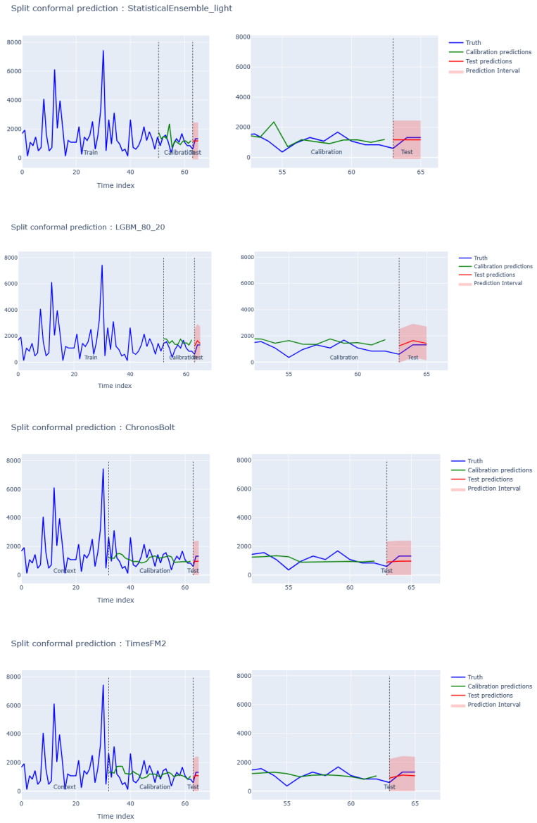
The central object is Split Conformal Prediction (SCP) with absolute-residual conformity scores and a user-set miscoverage rate, which splits each series into a context and a calibration set, computes the empirical quantile of the calibration residuals, and applies that quantile as a symmetric interval width around point forecasts. What carries the paper's claim is the interaction between zero-shot forecasting and this calibration split: TSFMs need only a context window (32 to 512 points), so the remaining historical data, up to roughly 94% of the series, is free for calibration, while classical learners like LightGBM give up 20% to 80% of the same data for training and lag creation. The paper uses a rolling-window scheme for TSFM calibration and reports local (per-series) quantiles as the headline results, with global quantiles deferred to the appendix.

What would settle it

Take a single non-stationary series (for example the hourly ERCOT data) and compute SCP intervals using a random split of the historical window versus a time-ordered split of the same window; if the empirical coverage differs substantially between the two splits, exchangeability fails and the reported model rankings in coverage cannot be attributed to the models themselves.

Watch

Extended reading notes

Core claim

On its own terms, the paper's claim is that in a split conformal prediction (SCP) framework with a target 90% coverage, zero-shot TSFMs—Chronos, Chronos-Bolt, TimesFM, TimesFM 2.0, and Lag-Llama—produce prediction intervals that are both narrower (lower MSIW) and better calibrated (closer to MCR around 90%) than statistical and gradient-boosting baselines when the historical data available for training and calibration is limited. The mechanism the paper identifies is compositional: the zero-shot property removes the training-set requirement, so a TSFM uses a short context and assigns the remaining data (for example 1720 to 8248 points on ERCOT, or 791 minus context minus horizon on NN5 Daily) entirely to calibration, whereas LightGBM must consume 20% to 80% of the same data for fitting and for lag creation. As data shrink, the paper argues, the calibration quantile estimate becomes imprecise and classic models degrade, so the gap is most pronounced in the smallest-data settings. The paper reports the effect holds across horizons and data frequencies, and that larger TSFMs performed better, suggesting the scaling rule has not plateaued.

Load-bearing premise

The coverage guarantee of split conformal prediction rests on the calibration residuals being exchangeable with the residuals that appear at prediction time, and the paper states plainly that its own time-series data do not satisfy this exchangeability, so differences in coverage across models may reflect the violation rather than genuine reliability.

Editorial extensions

If this is right

In data-scarce forecasting tasks, TSFMs become a natural default base model for split conformal prediction, since they free nearly all data for calibration.
The claimed advantage grows as available data shrinks, so the regime where classic models need the most training data is exactly where TSFM-based intervals should be preferred.
Because TSFM intervals are built on larger calibration sets, the quantile threshold is more stable across rolling windows, reducing variability in interval width.
Improved point accuracy of TSFMs translates into narrower intervals at the same coverage level, since the conformal width is driven by the magnitude of calibration residuals.
Larger TSFMs (more parameters) gave better results, implying further scaling could widen the gap over classical methods in conformal prediction settings.

Reading between the lines

Editorial extensions of the paper, not claims the author makes directly.

If the result holds, a testable extension is replacing SCP with a time-series-aware conformal method, such as adaptive conformal inference or ensemble batch prediction intervals, on top of the same TSFM forecasts; the paper's own exchangeability caveat suggests coverage gains could be more honest or even larger there.
The context-length versus calibration-fraction trade-off the paper leaves open could be quantified by sweeping the context size against the calibration fraction; TSFMs may tolerate much shorter contexts than the 128- or 512-point windows used here, and the optimal split is likely data-dependent.
The paper does not probe the extreme tail of scarcity, where a TSFM's context window (as low as 32 points) consumes most of the available history; in that regime a classical model trained on the full series could plausibly win, and mapping that threshold would sharpen the practical guidance.

Share X Bluesky LinkedIn Reddit HN

Editorial analysis

A structured set of objections, weighed in public.

Desk editor's note, referee report, and a circularity audit.

Desk Editor's Note

read the letter

Two things to know. First, this is the first side-by-side comparison I've seen of split conformal prediction running on Chronos, TimesFM, Lag-Llama plus classical baselines; that alone makes it useful for applied forecasting under data scarcity. Second, the central claim — TSFMs give more reliable conformalized intervals when data is limited because zero-shot prediction frees data for calibration — is plausible but not yet established. The biggest risk is the unverified zero-shot premise.

Where credit is due: the experimental setup is transparent. The configuration tables give exact train/calibration splits per model per dataset, and the rolling-window calibration scheme is clearly described. The authors also openly concede in Sections 4.4 and 6 that the data violate the exchangeability assumption SCP relies on; they know the finite-sample coverage guarantee does not strictly hold. The repeated finding that TSFMs beat the baselines on MASE while producing narrower intervals is a real empirical signal, and the gap widening as data shrinks is consistent with the tables.

Soft spots, in order of severity. First, the zero-shot premise is load-bearing and unverified. Section 2 asserts the models "have never seen the benchmarking datasets," with no evidence. M3 Monthly — the most data-scarce case where TSFMs look best — is a public benchmark that plausibly sits in Chronos's and TimesFM's pretraining corpora. If so, the M3 advantage is memorization, not zero-shot generalization. This is falsifiable by checking data manifests and rerunning after exclusion, but as it stands the abstract's causal claim ("more reliable ... thanks to their superior predictive accuracy") overreaches. Second, the reliability claim is undercut by the coverage rates themselves: Chronos lands at 82.7% on ERCOT-8760-S, and several other TSFM settings miss the 90% target. With the exchangeability violation conceded, those coverage numbers cannot carry the weight the conclusions place on them. The honest reading is "tighter intervals with often-but-not-always adequate coverage." Some of the comparison also builds the advantage in — TSFMs get nearly all data for calibration while LGBM must reserve training data — and while the paper is upfront about it, the headline numbers mix model accuracy with data allocation. Third, no variance or confidence intervals are reported on any aggregate; the twenty ERCOT windows are averaged bare, and NN5/M3 are single passes. Near the coverage boundary, those differences could be noise. Minor: the code-availability statement points to GitHub with no link, and typos like "zero-sot" suggest a rushed final pass.

Who this is for: practitioners doing uncertainty quantification in data-scarce forecasting, and people benchmarking TSFMs. It deserves serious peer review — the question is timely and the comparison is genuinely new. My recommendation: send it to review, but make acceptance contingent on verifying the zero-shot claim and either fixing the coverage shortfalls or softening the reliability language.

Referee Report

4 major / 6 minor

Summary. The manuscript compares time-series foundation models (Chronos, Chronos-Bolt, TimesFM, TimesFM 2.0, Lag-Llama) against classical baselines (Naive, Seasonal Naive, StatisticalEnsemble light, LightGBM with three train/calibration splits) in a split conformal prediction framework. Using four public datasets (ERCOT, NN5 Daily, NN5 Weekly, M3 Monthly) at short, medium, and long horizons, it reports mean coverage rate (MCR), mean scaled interval width (MSIW), and mean absolute scaled error (MASE). The central claim is that TSFMs give more reliable conformalized prediction intervals in data-constrained settings because they require almost no training data, leaving more data for calibration, and that this advantage grows as data become scarcer. The paper also includes a discussion of limitations, an appendix with detailed result tables, and states that all reproduction code is available.

Significance. If the central claim were fully supported, the practical recommendation—prefer zero-shot TSFMs as base forecasters in split conformal prediction when data are scarce—would be immediately useful and actionable. The paper is transparent about its limitations, ships code, and evaluates multiple frequencies, horizons, and model families. However, the evidence as presented does not yet establish the claim. Coverage shortfalls, the acknowledged violation of exchangeability, and the unverified zero-shot premise leave the observed advantage confounded. The paper does make a worthwhile contribution by identifying the data-allocation trade-off in conformal prediction with foundation models, but the supporting experiments need strengthening before the conclusions can be accepted.

major comments (4)

[Section 4.4, Table 5] Several TSFM configurations fail to reach the 90% target coverage (e.g., Chronos 82.7%, ChronosBolt 86.3%, TimesFM2 85.8% in ERCOT-8760-S; Chronos 81.7%, ChronosBolt 83.8%, TimesFM 87.4%, TimesFM2 83.2% in ERCOT-8760-M; Chronos 83.9%, TimesFM2 82.8% in ERCOT-8760-L), yet the text concludes in favor of TSFMs 'for the overall prediction.' The claim of 'more reliable' intervals requires an explicit criterion that accounts for coverage shortfalls, and reporting point MCR without standard errors or confidence intervals (20 windows are aggregated without variance) is insufficient to distinguish genuine reliability from calibration luck.
[Sections 4.4 and 6] The authors state that the data do not satisfy the exchangeability criterion of SCP: 'We argue that the coverage rate was not met because the data do not satisfy the exchangeability criterion of SCP' and 'our data do not meet the exchangeability criteria that guarantee marginal coverage.' Under non-exchangeability, the finite-sample marginal coverage guarantee of split conformal prediction is void, so coverage differences between models cannot be interpreted as reliability differences. The paper should either use conformal methods designed for time series (e.g., ACI, EnbPI, CQR) or justify why SCP remains valid under the rolling-window protocol used in Section 4.2.
[Section 2 and Section 4.1] The claim that the TSFMs 'have never seen the benchmarking datasets' is load-bearing for the zero-shot interpretation, but it is not verified. Public pretraining corpora for Chronos and TimesFM include broad open benchmarks such as M3; if M3 Monthly (66 points per series) overlapped with pretraining, the TSFM advantage on M3 reported in Table 6 would reflect memorization rather than zero-shot reliability. The authors should inspect the models' data manifests and rerun the analysis after excluding any overlapping pretraining datasets.
[Tables 3 and 4] The experimental design confounds model class with calibration-set size. TSFMs are allocated nearly all observations to calibration (e.g., 8248/8760 points in ERCOT-8760 and 1720/2232 points in ERCOT-2232), while LGBM and StatisticalEnsemble light must reserve 20–80% of data for training. Consequently, the second claimed advantage—'the calibration process is more stable because more data are used for calibration'—is partly true by construction and does not demonstrate an intrinsic property of TSFMs. A controlled comparison with equal calibration sizes across model classes, or with classical models trained on a separate external dataset, is needed to support the causal claim in the abstract.

minor comments (6)

[Throughout] There are numerous typographical errors and inconsistencies, including 'zero-sot' (Section 1), 'resons' (Section 2), 'againt' (Section 4.2), 'primarly' (Section 3), 'montly' (Section 4.5), 'Morever' (Abstract), 'M ISW' (Section 4.3.2), and the inconsistent notation 'maenaive,j' vs. 'M AEnaive,j' in Eq. (8).
[Eq. (1)] The definition of the adjusted miscoverage rate 1−α̂ = ⌈(|Cal|+1)(1−α)⌉/|Cal| should be clarified: as written, it appears to set the effective miscoverage level rather than the quantile index. The relationship to the standard SCP quantile (e.g., the ⌈(|Cal|+1)(1−α)⌉-th smallest conformity score) should be spelled out.
[Section 4.4] The StatisticalEnsemble light model is omitted from the ERCOT-8760 experiments 'due to time constraints,' but this is only mentioned in the prose; the tables mark the entries with 'x.' This omission should be stated more prominently in the experimental setup and in the table captions.
[Appendix C] Cross-references to appendix tables are imprecise: Section 4.4 refers to 'Table 5 in the Appendix' and Section 4.5 refers to 'Table 6 in Appendix,' but the tables are in Appendix C and the numbering depends on the final layout. Please use automatic cross-references or explicit appendix labels.
[References] The reference to 'Angelopoulos and Bate' should be updated to the published version or cite the arXiv identifier consistently; the 'Nixla' entry is incomplete and appears to contain a typo.
[Section 6] The acknowledged limitation about context-length choice is important; a small sensitivity analysis varying the context/calibration split would help quantify how much the conclusions depend on this choice.

Circularity Check

1 steps flagged · score 4.0 of 10

No self-citation or fitted-prediction circularity; the 'stable calibration' headline advantage is the experimental data split itself, making the paper only partially circular.

self definitional [Abstract (second claimed advantage); Section 4.2, Tables 3 and 4; Section 6 (Discussion)]
"Second, the calibration process is more stable because more data are used for calibration. Morever, the fewer data available, the more pronounced these benefits become, as classic models require a substantial amount of data for effective training."

The claimed stability advantage is entailed by the authors' own data allocation rather than measured. In Tables 3 and 4, TSFMs receive 512 context points (or 128/64/32) and nearly all remaining points for calibration (e.g., 8248 of 8760 ERCOT points), while classic models must hold out training data (StatisticalEnsemble 7008 fit / 1752 calibration; LGBM8020 80% fit / 20% calibration). The attribution 'more stable because more data are used for calibration' reduces the advantage to this protocol split: the cause invoked is precisely the design choice, and no experiment varies the calibration share for TSFMs (e.g., 20% calibration) to test whether stability is a property of TSFMs or just of calibration-set size.

full rationale

This is an empirical benchmark paper rather than a derivation, so most circularity patterns do not apply. There are no self-citations by the present authors (Achour, Bouher, Nguyen, Chesneau) among the references; no uniqueness theorem is imported from prior work by the same group; no ansatz is smuggled in via citation; and no known result is renamed. The central reliability claim (TSFMs give more reliable conformalized intervals in data-constrained settings thanks to superior predictive accuracy) rests on held-out measurements (MASE, MCR, MSIW) that are genuinely independent of the model inputs, and the MASE advantage is a real empirical outcome. The one reduction-by-construction element is the second headline advantage: 'the calibration process is more stable because more data are used for calibration.' Because the larger calibration set for TSFMs is the authors' own allocation (Tables 3-4), this advantage is a restatement of the experimental protocol rather than an independently demonstrated property. The first advantage retains independent empirical content, so the paper is only partially circular, not wholly so. The self-admitted violation of exchangeability (Sections 4.4 and 6: 'our data do not meet the exchangeability criteria that guarantee marginal coverage') is a correctness/validity risk for the coverage-guarantee interpretation, not a circularity, and the zero-shot or data-contamination question raised by external reviewers is an external falsifiability concern, not a circularity; neither raises the score further.

Assumptions & free parameters 2 free parameters · 2 assumptions · 0 invented entities

The paper introduces no new entities and fits no statistical parameters; the listed free parameters are experimental design choices that influence the comparison. The central claim rests on the exchangeability assumption of SCP and on the zero-shot status of the TSFMs, both imperfectly satisfied.

free parameters (2)

context_length = 512, 128, 64, or 32 depending on dataset
Chosen as a multiple of 32 and set to 512 when data allow, reduced to 32 in the worst case (Table 4). This choice affects how much history TSFMs see and how many points remain for calibration, and the paper notes the trade-off is not fully explored (Section 6).
LGBM train/calibration split = 80/20, 50/50, 20/80
Ad hoc ratios chosen to illustrate the training/calibration trade-off; results differ noticeably across these ratios, especially in the ERCOT-2232 setting.

assumptions (2)

domain assumption Calibration and test residuals are exchangeable enough for split conformal prediction to provide its finite-sample coverage guarantee.
The validity of SCP intervals (Eq. 2) depends on exchangeability; the authors explicitly note the data violate this criterion in Section 4.4 and in the Discussion.
domain assumption The evaluated TSFMs are zero-shot with respect to the benchmark datasets.
The claim that no training data is required rests on the models not having seen ERCOT, NN5, and M3 during pretraining; asserted for three base models, while training data for Chronos-Bolt and TimesFM2 is listed as unknown (Table 2).

how reviews work

0 comments

Cite this review

Pith. "Pith review of Foundation models for time series forecasting: Application in conformal prediction." pith.science (2026). https://pith.science/paper/GTLEQELK

@misc{pith2026250708858,
  author       = {Pith},
  title        = {Pith review of: Foundation models for time series forecasting: Application in conformal prediction},
  year         = {2026},
  howpublished = {\url{https://pith.science/paper/GTLEQELK}},
  note         = {Machine review of arXiv:2507.08858}
}

read the original abstract

The zero-shot capabilities of foundation models (FMs) for time series forecasting offer promising potentials in conformal prediction, as most of the available data can be allocated to calibration. This study compares the performance of Time Series Foundation Models (TSFMs) with traditional methods, including statistical models and gradient boosting, within a conformal prediction setting. Our findings highlight two key advantages of TSFMs. First, when the volume of data is limited, TSFMs provide more reliable conformalized prediction intervals than classic models, thanks to their superior predictive accuracy. Second, the calibration process is more stable because more data are used for calibration. Morever, the fewer data available, the more pronounced these benefits become, as classic models require a substantial amount of data for effective training. These results underscore the potential of foundation models in improving conformal prediction reliability in time series applications, particularly in data-constrained cases. All the code to reproduce the experiments is available.

Figures

Figures reproduced from arXiv: 2507.08858 by the authors.

**Figure 1.** Rolling window. Let C the context size and H the prediction length. We use the first C available data points as the context to predict H points {yˆC+1, ...yˆC+H}. The window is then shifted forward by H steps to predict the next set of points {yˆC+H+1, ...yˆC+2H}. This process continues until only r data points remain, where 0 ≤ r < H. In the final step, H points are forecasted with context C, but only the first r p… view at source ↗

**Figure 2.** Illustration of prediction interval. The light blue lines represent the upper and lower [PITH_FULL_IMAGE:figures/full_fig_p008_2.png] view at source ↗

**Figure 3.** Window sampling - Scenario 1 Model ERCOT 8760 points ERCOT 2232 points Points for context/fit Points for calibration Points for context/fit Points for calibration Naive 1 8759 1 2231 SeasonalNaive h 8760-h h 2232-h StatisticalEnsemble.light 7008 1752 1785 447 LGBM 20 80 0.2x(8760-h-168) 0.8x(8760-h-168) 0.2x(2232-h-168) 0.8x(2232-h-168) LGBM 50 50 0.5x(8760-h-168) 0.5x(8760-h-168) 0.5x(2232-h-168) 0.5x(2232-h-168) L… view at source ↗

Figures from the paper (10 more)

**Figure 4.** Figure 4: Split conformal prediction results on ERCOT 8760. Better models are those appear to [PITH_FULL_IMAGE:figures/full_fig_p010_4.png]

**Figure 5.** Figure 5: Split conformal prediction on ERCOT 2232 [PITH_FULL_IMAGE:figures/full_fig_p011_5.png]

**Figure 6.** Figure 6: Split conformal prediction on 2232 points of ERCOT - horizon S - with StatisticalEnsem [PITH_FULL_IMAGE:figures/full_fig_p013_6.png]

**Figure 7.** Figure 7: Split conformal prediction on NN5 Daily The conclusions remain consistent across different horizons, which enhances the robustness of the insights derived above. 5 Related work Recent successes of FMs in NLP, CV and multimodal (C. Zhou et al., 2024) have catalyzed sign…

**Figure 8.** Figure 8: Split conformal prediction on NN5 Weekly [PITH_FULL_IMAGE:figures/full_fig_p015_8.png]

**Figure 9.** Figure 9: Split conformal prediction on M3 Monthly [PITH_FULL_IMAGE:figures/full_fig_p016_9.png]

**Figure 10.** Figure 10: Examples of split conformal prediction made by different models on one time series in [PITH_FULL_IMAGE:figures/full_fig_p017_10.png]

**Figure 11.** Figure 11: Examples of split conformal prediction made by different models on one time series in [PITH_FULL_IMAGE:figures/full_fig_p018_11.png]

**Figure 12.** Figure 12: Examples of split conformal prediction made by different models on one time series in [PITH_FULL_IMAGE:figures/full_fig_p019_12.png]

**Figure 13.** Figure 13: Datasets distribution B Normalized interval width for global quantiles Global quantiles are used only in the context of multivariate datasets, namely NN5 daily, NN5 weekly, and M3 Monthly. We obtain one interval width which are l for a given model and lnaive with the …

Discussion (0). Sign in to comment.

Reference graph

Works this paper leans on

3 extracted references · 1 canonical work pages

[1]

Abbass, K., Qasim, M., Song, H., Murshed, M., Mahmood, H., & Younis, I. (2022). A review of the global climate change impacts, adaptation, and sustainable mitigation measures. Environ- mental Science and Pollution Research. https://doi.org/10.1007/s11356-022-19718-6 Aksu, T., Woo, G., Liu, J., Liu, X., Liu, C., Savarese, S., Xiong, C., & Sahoo, D. (2024)....

arXiv 2022
[7]

23 Horizon Model ERCOT 8760 points ERCOT 2232 points MASE MCR IW MSIW MASE MCR IW MSIW S Naive 1.000 87.5 15946 1.000 1.000 87.9 15160 1.000 SeasonalNaive 0.795 91.7 5504 0.461 1.338 79.2 6742 0.882 Stat.Ensemblelight x x x x 1.018 87.9 6119 0.801 LGBM20 80 0.592 96.7 10748 0.708 1.195 89.2 9328 0.724 LGBM50 50 0.580 89.8 7869 0.511 0.841 87.9 7266 0.559 ...

work page
[30]

Khurana, D., Koli, A., Khatter, K., & Singh, S. (2022). Natural language processing: State of the art, current trends and challenges. Multimedia Tools and Applications , 82(3), 3713–3744. https://doi.org/10.1007/s11042-022-13428-4 Kolassa, S., Rostami-Tabar, B., & Siemsen, E. (2023). Demand forecasting for executives and pro- fessionals. CRC Press. https:...

arXiv 2022

Pith tools

Reviewed August 6, 2026 · model on record in the stance chip above.

[1] [1]

Abbass, K., Qasim, M., Song, H., Murshed, M., Mahmood, H., & Younis, I. (2022). A review of the global climate change impacts, adaptation, and sustainable mitigation measures. Environ- mental Science and Pollution Research. https://doi.org/10.1007/s11356-022-19718-6 Aksu, T., Woo, G., Liu, J., Liu, X., Liu, C., Savarese, S., Xiong, C., & Sahoo, D. (2024)....

arXiv 2022

[2] [7]

23 Horizon Model ERCOT 8760 points ERCOT 2232 points MASE MCR IW MSIW MASE MCR IW MSIW S Naive 1.000 87.5 15946 1.000 1.000 87.9 15160 1.000 SeasonalNaive 0.795 91.7 5504 0.461 1.338 79.2 6742 0.882 Stat.Ensemblelight x x x x 1.018 87.9 6119 0.801 LGBM20 80 0.592 96.7 10748 0.708 1.195 89.2 9328 0.724 LGBM50 50 0.580 89.8 7869 0.511 0.841 87.9 7266 0.559 ...

work page

[3] [30]

Khurana, D., Koli, A., Khatter, K., & Singh, S. (2022). Natural language processing: State of the art, current trends and challenges. Multimedia Tools and Applications , 82(3), 3713–3744. https://doi.org/10.1007/s11042-022-13428-4 Kolassa, S., Rostami-Tabar, B., & Siemsen, E. (2023). Demand forecasting for executives and pro- fessionals. CRC Press. https:...

arXiv 2022