REVIEW 5 major objections 6 minor 37 references
Discovering Governing Equations in the Presence of Uncertainty
T0 review · 5 major / 6 minor · reviewed 2026-08-06 · deepseek-v4-flash
Pith's one-line read Treating unknown coefficients as random variables, not fixed numbers, recovers governing equations from noisy variable data with quantified uncertainty.
desk verdict Plausible extension of stochastic inverse modeling to physics discovery, but the manuscript omits all its empirical evidence and never specifies the candidate libraries, so the headline 82% RMSE claim cannot be verified. read the letter →
The pith
A machine-rendered reading of the paper's core claim, the machinery that carries it, and where it could break.
The reading
What carries the argument
The load-bearing object is the push-forward acceptance ratio $\varphi(\hat Q(\lambda))=\pi_Y(\hat Q(\lambda)|Y)/\pi_Q(\hat Q(\lambda))$: the likelihood of a simulated trajectory under a kernel-density estimate of the observed data, divided by the push-forward density of prior samples through the candidate equation. Rejection sampling against this ratio converts prior coefficient draws into posterior samples whose simulated trajectories match the empirical data distribution. Around this ratio, the machinery includes sparsity-promoting priors (spike-and-slab and regularized horseshoe) to zero out inactive library terms, a matched-block bootstrap that manufactures dependent sample paths when only one trajectory exists, and a rule-of-thumb bandwidth for the kernel-density likelihood.
What would settle it
Run SIP on a synthetic dynamical system whose true equation includes a term deliberately omitted from the candidate library (e.g., a cubic $x^3$ term not offered in $\Theta(X)$); the central claim is refuted if the recovered equations claim to match the data while missing that term, or if the 95% credible intervals fail to cover trajectories generated from the true model.
Extended reading notes
Core claim
The paper's central claim is that the data-generating process is $Y=\int \lambda\Theta(X)\,dt+\epsilon$ with $\epsilon\sim N(0,\sigma^2)$, where the coefficient matrix $\lambda$ is not a fixed parameter but a random quantity encoding input or system variability. The stochastic inverse problem is solved by selecting a measure $\mu_\Lambda^*=\arg\min_{\mu_\Lambda} D_{\mathrm{KL}}(\hat\mu_Y\|\mu_Y)$ so that simulating prior samples through the candidate equations pushes the coefficient distribution forward onto the observed data distribution. The posterior over coefficients takes the push-forward Bayes-like form $\pi_\Lambda(\lambda|Y)=\pi_\Lambda(\lambda)\,\pi_Y(\hat Q(\lambda)|Y)/\pi_Q(\hat Q(\lambda))$, with sparsity-promoting priors shrinking irrelevant library terms to zero, matched-block bootstrap generating multiple dependent sample paths from a single trajectory, and rejection sampling drawing posterior samples. The paper reports that this consistently identifies the correct equations and recovers coefficient distributions whose 95% credible intervals track observed trajectories across all benchmarks, with an average 82% reduction in coefficient RMSE relative to SINDy and its Bayesian variant.
Load-bearing premise
The load-bearing premise is that the candidate physics library $\Theta(X)$ for each case study contains the exact true dynamics terms; the paper never lists these libraries in Section 3, so the method could be selecting among pre-known correct terms, and if the true term is absent, no sampling scheme can recover it.
Editorial extensions
If this is right
- On noisy and variable data, SIP recovers the true active physics terms where SINDy and its Bayesian variant add spurious terms or drop real ones.
- The recovered coefficient posteriors give 95% credible intervals that track observed trajectories, so predictions can be reported with calibrated uncertainty.
- A single observed trajectory suffices: the matched-block bootstrap creates synthetic paths that preserve temporal dependence, extending the method to historical or unrepeatable experiments.
- The approach works for chaotic systems and real experimental fluids, suggesting broad applicability across biology and engineering.
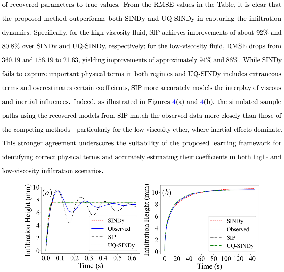
- Coefficient RMSE drops by about 82% on average, with per-case improvements up to roughly 99% over SINDy and 96% over the Bayesian variant, so the accuracy gain is not limited to one example.
Reading between the lines
- If system variability is real, more data will not shrink coefficient posterior uncertainty to zero; the framework implies an irreducible uncertainty floor set by input variability, a phenomenon standard Bayesian discovery cannot express.
- A natural stress test the paper does not run: apply SIP with an intentionally incomplete or misspecified library and ask whether the KL-minimizing push-forward degrades gracefully (wide credible intervals, flagged missing terms) or silently substitutes spurious terms.
- A testable extension separating measurement-noise variance $\sigma^2$ from coefficient variability could let practitioners quantify what fraction of observed dispersion is intrinsic system variability versus observation error; the paper lists disentangling these as future work.
- Because the acceptance ratio relies on kernel density estimates, performance may degrade sharply as the state or parameter dimension grows; comparing acceptance rates and accuracy against dimension would probe scalability.
Editorial analysis
A structured set of objections, weighed in public.
Referee Report
Summary. The manuscript proposes a stochastic inverse physics-discovery (SIP) framework for identifying governing differential equations from noisy, variable, and data-limited observations. The unknown coefficients are treated as random variables with sparsity-promoting priors, and their posterior is inferred by minimizing the KL divergence between the push-forward of simulated trajectories and the empirical data distribution; a matched-block bootstrap is used when only a single trajectory is available. The method is benchmarked on simulated Lotka–Volterra, the Hudson Bay lynx–hare data, the Lorenz system, and fluid-infiltration experiments, with the reported headline result being an average 82% reduction in coefficient RMSE relative to SINDy and UQ-SINDy.
Significance. If the reported results are substantiated, the paper would offer a useful and timely extension of equation-discovery methods to settings with input variability and limited data, and the use of matched-block bootstrap for single-trajectory likelihood estimation is a sensible component. However, the central empirical claims are not verifiable from the submitted manuscript because the results table and all figures are missing, and several methodological details that are load-bearing for the claims remain unspecified. The potential significance is therefore real but cannot be assessed at this stage.
major comments (5)
- [Section 3, Table 1 and Figures 1–4] Table 1 is present only as a header with no content, and Figures 1–4, which are referenced throughout Sections 3.1–3.4, are absent from the manuscript. Every quantitative claim in the paper—the average 82% RMSE reduction, the per-case improvement percentages, the recovered coefficient distributions, and the posterior-predictive coverage—is tied to these missing exhibits. The abstract's headline result cannot be checked, and the comparison with SINDy and UQ-SINDy is not reproducible as submitted.
- [Section 3 and Eq. (2)] The candidate library Theta(X) is never specified for any of the four case studies, even though structural recovery in Eq. (2) is exactly a selection of nonzero coefficients from this library. Without knowing whether the true terms (e.g., uv in Lotka–Volterra, xz and xy in Lorenz, or the inertial-capillarity terms in infiltration) were included and how many distractor terms were present, the claim that SIP 'consistently identifies the correct equations' may amount to selection among pre-specified correct terms rather than discovery. The lynx–hare figure caption lists a library {1,u,v,uv}, but the same information is not given for the other studies.
- [Section 3.2] For the Hudson Bay lynx–hare data, the manuscript reports RMSE 'relative to the ground truth model coefficients' and compares the recovered distributions to 'ground truth' in Figure 2, but this is observational data with no known coefficient values. The ground truth used for these calculations is never defined. Without a clearly stated reference solution (for example, coefficients calibrated by an independent method or taken from a specific ecological study), the reported RMSE reductions of 45–80% for this case are not interpretable.
- [Section 2.4, Eqs. (11)–(12)] The claimed consistency guarantee is not established in the manuscript. Theorem 1 is stated with a proof outsourced to [29], and Theorem 2 is a restatement of a result from [34] with 'Refer to [34] for details and proof.' Eq. (11) contains undefined objects, and Eq. (12) uses the notation μ_{\hat Q(μ_Λ)}^Y and \hat Q^{-1} without definition. The text says 'We subsequently provide the theoretical analysis,' but no derivation, precise assumptions, or connection to the finite-sample rejection sampler in Algorithm 1 is given. If a consistency guarantee is part of the paper's contribution, it needs to be stated in a self-contained and correct form.
- [Section 2.1, likelihood expression and bandwidth] The kernel-density likelihood is not well defined as written. In the expression for \hatπ_Y(Q(λ)|Y), the quantity ([Y_i]_j - [\hat Y]_j)^2 is a vector of length n, so the exponential is not scalar unless a norm is intended; the authors should specify the norm and the bandwidth units. In addition, the bandwidth rule h ∝ r^{-1/(n+4)} follows Scott's rule for a sample of size r in dimension n, treating the time-series length as the KDE dimension, which is an unusual and potentially degenerate choice for long trajectories. Since this likelihood is used in all posterior computations, the sensitivity of the results to this choice should be discussed.
minor comments (6)
- [Algorithm 1] The word 'Algortihm' is misspelled in the text preceding Algorithm 1.
- [Eq. (6)] The symbol \Q(λ) used in Eq. (6) and elsewhere is not defined; it should be the candidate solution Q(λ).
- [Section 3.2 and Figure 3] The text states the Hudson Bay dataset spans 20 years, while the caption for Figure 3 places year 0 at 1900 and the standard dataset is commonly cited as a much longer record; please clarify the exact time interval used.
- [References] References [10] and [12] are the same paper (Brunton et al., 2016); one should be removed or the citations consolidated.
- [Conclusion] The conclusion states that improvements 'often exceed 90%' while the abstract reports an average of 82%; please reconcile these statements and report the range of per-case improvements.
- [Reproducibility] No code or data availability statement is included; providing the candidate libraries, code, and processed data would substantially improve reproducibility.
Circularity Check
No significant circularity found; the methodological core is externally cited and the empirical benchmarks are independent.
full rationale
The paper's inference machinery is explicitly adopted from external prior work: the posterior formula (Eq. 6) is attributed to Butler et al. [26], and the consistency Theorem 2 is credited to [34] with proof outsourced. Neither citation is self-referential, and the paper does not claim to derive these results from scratch; it uses them as building blocks. The empirical comparisons to SINDy and UQ-SINDy on simulated, historical, and experimental data are external benchmarks, not fitted redefinitions. The abstract's '82% RMSE reduction' is a comparison against standard baselines, not a quantity that is equivalent to an input by construction. The absence of explicit candidate libraries is a reporting limitation that affects interpretability but does not constitute circularity: the library is a standard input to SINDy-type methods, and the paper does not define its recovered equations in terms of the library itself. The two self-citations ([24], [36]) are peripheral data/context references and are not load-bearing for the central argument. No step reduces, by definition or by self-citation, to its own inputs.
Assumptions & free parameters
free parameters (4)
- KDE bandwidth h =
Scott's rule or manually set
- Matched block bootstrap block length l
- Number of prior samples N
- Prior hyperparameters
assumptions (4)
- domain assumption Measurement noise is additive, zero-mean Gaussian (Eq. 4)
- standard math The stochastic inverse posterior formula (Eq. 6) is valid
- standard math The matched-block bootstrap is consistent (Theorem 1)
- ad hoc to paper The candidate library Theta(X) contains the true governing terms
Cite this review
Pith. "Pith review of Discovering Governing Equations in the Presence of Uncertainty." pith.science (2026). https://pith.science/paper/TCBGXO5P
@misc{pith2026250709740,
  author       = {Pith},
  title        = {Pith review of: Discovering Governing Equations in the Presence of Uncertainty},
  year         = {2026},
  howpublished = {\url{https://pith.science/paper/TCBGXO5P}},
  note         = {Machine review of arXiv:2507.09740}
}
read the original abstract
In the study of complex dynamical systems, understanding and accurately modeling the underlying physical processes is crucial for predicting system behavior and designing effective interventions. Yet real-world systems exhibit pronounced input (or system) variability and are observed through noisy, limited data conditions that confound traditional discovery methods that assume fixed-coefficient deterministic models. In this work, we theorize that accounting for system variability together with measurement noise is the key to consistently discover the governing equations underlying dynamical systems. As such, we introduce a stochastic inverse physics-discovery (SIP) framework that treats the unknown coefficients as random variables and infers their posterior distribution by minimizing the Kullback-Leibler divergence between the push-forward of the posterior samples and the empirical data distribution. Benchmarks on four canonical problems -- the Lotka-Volterra predator-prey system (multi- and single-trajectory), the historical Hudson Bay lynx-hare data, the chaotic Lorenz attractor, and fluid infiltration in porous media using low- and high-viscosity liquids -- show that SIP consistently identifies the correct equations and lowers coefficient root-mean-square error by an average of 82\% relative to the Sparse Identification of Nonlinear Dynamics (SINDy) approach and its Bayesian variant. The resulting posterior distributions yield 95\% credible intervals that closely track the observed trajectories, providing interpretable models with quantified uncertainty. SIP thus provides a robust, data-efficient approach for consistent physics discovery in noisy, variable, and data-limited settings.
Figures


Figures from the paper (1 more)
Reference graph
Works this paper leans on
-
[29]
Matched-block bootstrap for dependent data,
E. Carlstein, K.-A. Do, P. Hall, T. Hesterberg, and H. R. Künsch, “Matched-block bootstrap for dependent data,”Bernoulli, vol. 4, no. 3, pp. 305–328, 1998
work page 1998
-
[34]
Data-consistent inversion for stochastic input-to- output maps,
T. Butler, T. Wildey, and T. Y. Yen, “Data-consistent inversion for stochastic input-to- output maps,”Inverse Problems, vol. 36, no. 8, p. 085015, 2020
work page 2020
-
[1]
C. H. F. Peters, E. B. Knobel,et al., Ptolemy’s catalogue of stars: A revision of the Almagest, vol. 86. Carnegie Institution of Washington, 1915
work page 1915
-
[2]
C. Ptolemy and W. Donahue,The almagest: introduction to the mathematics of the heavens. Green Lion Press Santa Fe, NM, 2014
work page 2014
-
[3]
R. S. Westfall,Never at rest: A biography of Isaac Newton. Cambridge University Press, 1983
work page 1983
-
[4]
T. S. Kuhn,The structure of scientific revolutions, vol. 962. University of Chicago press Chicago, 1962
work page 1962
-
[5]
Stationary sequences in hilbert space,
A. Kolmogorov, “Stationary sequences in hilbert space,”Bulletin of the Academy of Sciences of the USSR, Mathematics Series, pp. 1–14, 1941
work page 1941
-
[6]
Wiener,Extrapolation, Interpolation, and Smoothing of Stationary Time Series
N. Wiener,Extrapolation, Interpolation, and Smoothing of Stationary Time Series. MIT Press, 1949. 21
work page 1949
Show all 37 references
-
[7]
Automated reverse engineering of nonlinear dynamical systems,
J. Bongard and H. Lipson, “Automated reverse engineering of nonlinear dynamical systems,” Proceedings of the National Academy of Sciences, vol. 104, no. 24, pp. 9943–9948, 2007
2007
-
[8]
Distilling free-form natural laws from experimental data,
M. Schmidt and H. Lipson, “Distilling free-form natural laws from experimental data,” Science, vol. 324, no. 5923, pp. 81–85, 2009
2009
-
[9]
Nonlinear dynamical system identification from uncertain and indirect measurements,
H. U. Voss, J. Timmer, and J. Kurths, “Nonlinear dynamical system identification from uncertain and indirect measurements,”International Journal of Bifurcation and Chaos, vol. 14, no. 06, pp. 1905–1933, 2004
1905
-
[10]
Discovering governing equations from data by sparse identification of nonlinear dynamical systems,
S. L. Brunton, J. L. Proctor, and J. N. Kutz, “Discovering governing equations from data by sparse identification of nonlinear dynamical systems,”Proceedings of the national academy of sciences, vol. 113, no. 15, pp. 3932–3937, 2016
2016
-
[11]
Machine learning for fluid mechanics,
S. L. Brunton, B. R. Noack, and P. Koumoutsakos, “Machine learning for fluid mechanics,” Annual Review of Fluid Mechanics, vol. 52, pp. 477–508, 2020
2020
-
[12]
Discovering governing equations from data by sparse identification of nonlinear dynamical systems,
S. L. Brunton, J. L. Proctor, and J. N. Kutz, “Discovering governing equations from data by sparse identification of nonlinear dynamical systems,”Proceedings of the National Academy of Sciences, vol. 113, no. 15, pp. 3932–3937, 2016
2016
-
[13]
A unified sparse optimization framework to learn parsimonious physics-informed models from data,
K. Champion, P. Zheng, A. Y. Aravkin, S. L. Brunton, and J. N. Kutz, “A unified sparse optimization framework to learn parsimonious physics-informed models from data,”IEEE Access, vol. 8, pp. 169259–169271, 2020
2020
-
[14]
Data-driven discovery of coordinates and governing equations,
K. Champion, B. Lusch, J. N. Kutz, and S. L. Brunton, “Data-driven discovery of coordinates and governing equations,”Proceedings of the National Academy of Sciences, vol. 116, no. 45, pp. 22445–22451, 2019
2019
-
[15]
Hidden physics models: Machine learning of nonlinear partial differential equations,
M. Raissi and G. E. Karniadakis, “Hidden physics models: Machine learning of nonlinear partial differential equations,”Journal of Computational Physics, vol. 357, pp. 125–141, 2018
2018
-
[16]
Hypersindy: Deep generative modeling of nonlinear stochastic governing equations,
M. Jacobs, B. W. Brunton, S. L. Brunton, J. N. Kutz, and R. V. Raut, “Hypersindy: Deep generative modeling of nonlinear stochastic governing equations,” 2023
2023
-
[17]
Generalizing the sindy approach with nested neural networks,
C. Fiorini, C. Flint, L. Fostier, E. Franck, R. Hashemi, V. Michel-Dansac, and W. Tenachi, “Generalizing the sindy approach with nested neural networks,” 2023. 22
2023
-
[18]
Sparsifying priors for bayesian uncertainty quantification in model discovery,
S. M. Hirsh, D. A. Barajas-Solano, and J. N. Kutz, “Sparsifying priors for bayesian uncertainty quantification in model discovery,”Royal Society Open Science, vol. 9, no. 2, p. 211823, 2022
2022
-
[19]
Ensemble-sindy: Robust sparse model discovery in the low-data, high-noise limit, with active learning and control,
U. Fasel, J. N. Kutz, B. W. Brunton, and S. L. Brunton, “Ensemble-sindy: Robust sparse model discovery in the low-data, high-noise limit, with active learning and control,” Proceedings of the Royal Society A, vol. 478, no. 2260, 2022
2022
-
[20]
Bayesian identification of dynamical systems,
R. K. Niven, A. Mohammad-Djafari, L. Cordier, M. Abel, and M. Quade, “Bayesian identification of dynamical systems,”Proceedings, 2019, MaxEnt 2019, p. 149, 2020
2019
-
[21]
Bindy–bayesian identification of nonlinear dynamics with reversible-jump markov-chain monte-carlo,
M. D. Champneys and T. J. Rogers, “Bindy–bayesian identification of nonlinear dynamics with reversible-jump markov-chain monte-carlo,”arXiv preprint arXiv:2408.08062, 2024
2024 arXiv
-
[22]
Impact of time varying interaction: Formation and annihilation of extreme events in dynamical systems,
S. Leo Kingston, G. Kumaran, A. Ghosh, S. Kumarasamy, and T. Kapitaniak, “Impact of time varying interaction: Formation and annihilation of extreme events in dynamical systems,” Chaos: An Interdisciplinary Journal of Nonlinear Science, vol. 33, no. 12, p. 123134, 2023
2023
-
[23]
State of the art in directed energy deposition: From additive manufacturing to materials design,
A. Dass and A. Moridi, “State of the art in directed energy deposition: From additive manufacturing to materials design,”Coatings, vol. 9, no. 7, p. 418, 2019
2019
-
[24]
Characterization of elastoplastic properties of additively manufactured specimens from indentation data using stochastic inverse mod- eling,
R. Olabiyi, J. Weaver, and A. Iquebal, “Characterization of elastoplastic properties of additively manufactured specimens from indentation data using stochastic inverse mod- eling,” in International Manufacturing Science and Engineering Conference, vol. 88100, p. V001T01A048, ...
2024
-
[25]
Spatial and temporal variability of soil moisture and its driving factors in the northern agricultural regions of china,
Z. Cheng, F. Wang, X. Mei, and D. Wu, “Spatial and temporal variability of soil moisture and its driving factors in the northern agricultural regions of china,”Water, vol. 16, no. 4, p. 556, 2024
2024
-
[26]
Combining push-forward measures and bayes’ rule to construct consistent solutions to stochastic inverse problems,
T. Butler, J. Jakeman, and T. Wildey, “Combining push-forward measures and bayes’ rule to construct consistent solutions to stochastic inverse problems,”SIAM Journal on Scientific Computing, vol. 40, no. 2, pp. A984–A1011, 2018
2018
-
[27]
Bayesian variable selection in linear regression,
T. J. Mitchell and J. J. Beauchamp, “Bayesian variable selection in linear regression,” Journal of the american statistical association, vol. 83, no. 404, pp. 1023–1032, 1988. 23
1988
-
[28]
Handling sparsity via the horseshoe,
C. M. Carvalho, N. G. Polson, and J. G. Scott, “Handling sparsity via the horseshoe,” in Artificial intelligence and statistics, pp. 73–80, PMLR, 2009
2009
-
[30]
Sindy-sa framework: enhancing nonlinear system identification with symmetry and conservation laws,
Z. Wang, X. Wang, Y. Wang, Y. Wang, Y. Wang, and Y. Wang, “Sindy-sa framework: enhancing nonlinear system identification with symmetry and conservation laws,”Nonlinear Dynamics, vol. 110, pp. 1–20, 2022
2022
-
[31]
D. W. Scott,Multivariate density estimation: theory, practice, and visualization. John Wiley & Sons, 2015
2015
-
[32]
Variable selection via gibbs sampling,
E. I. George and R. E. McCulloch, “Variable selection via gibbs sampling,”Journal of the American Statistical Association, vol. 88, no. 423, pp. 881–889, 1993
1993
-
[33]
Sparsity information and regularization in the horseshoe and other shrinkage priors,
J. Piironen and A. Vehtari, “Sparsity information and regularization in the horseshoe and other shrinkage priors,”Electronic Journal of Statistics, vol. 11, pp. 5018–5051, 2017
2017
-
[35]
C. G. Hewitt,The conservation of the wild life of Canada. New York: C. Scribner, 1921
1921
-
[36]
Multimodal boiling dataset with synchronized acoustic, optical, and thermal measurements under steady-state and transient heat loads,
H. Pandey, C. Li, and H. Hu, “Multimodal boiling dataset with synchronized acoustic, optical, and thermal measurements under steady-state and transient heat loads,”Data in Brief, vol. 55, p. 110582, 2024
2024
-
[37]
Inertial capillarity,
D. Quéré, “Inertial capillarity,”Europhysics Letters, vol. 39, no. 5, p. 533, 1997. 24
1997
Reviewed August 6, 2026 · model on record in the stance chip above.
Discussion (0). Continue with ORCID to comment.