REVIEW 3 major objections 5 minor 25 references
Efficient Decentralized Learning of Generalized Quantal Response Equilibrium
T0 review · 3 major / 5 minor · reviewed 2026-08-06 · deepseek-v4-flash
Pith's one-line read A decentralized learning rule provably drives a smoothed game gap to zero at rate O(log T/T), giving finite-time convergence to generalized quantal response equilibria.
desk verdict The algorithm is a reasonable extension and the bandit analysis is new, but the main theorem does not establish convergence to GQRE because the gap function vanishes on pure profiles and the iterates may approach the boundary. read the letter →
The pith
A machine-rendered reading of the paper's core claim, the machinery that carries it, and where it could break.
The reading
What carries the argument
The load-bearing object is the smoothed gap function $V(\pi)$, a regularized analogue of the Nash gap that serves as the Lyapunov function of the proof. For each player, $V_i(\pi) = \max_{s \in \Delta(A_i)} \langle s - \pi_i, \nabla_{\pi_i} u_i^{f_i}(\pi)\rangle - \eta \, \mathrm{KL}(s, \pi_i)$, which the Donsker-Varadhan variational formula evaluates in closed form as $\eta \log \langle \pi_i, \exp(\nabla u_i^{f_i}/\eta)\rangle - \langle \pi_i, \nabla u_i^{f_i}\rangle$, and it is zero exactly at the GQRE on fully mixed profiles. The update that makes the gap drift downward is the KL-smoothed Frank-Wolfe direction $s_i^*(\pi) = \arg\max_{s} \langle s, \nabla u_i^{f_i}\rangle - \eta \, \mathrm{KL}(s, \pi_i)$, a softmax over actions, followed by projection onto the $\epsilon_t$-exploration simplex $\Delta(A_i; \epsilon_t)$ so every action keeps probability at least $\epsilon_t$. The noise is controlled by taking $M_t = \lceil 1/(\epsilon_t \gamma_t^2)\rceil$ samples per step, which keeps the bandit gradient estimator, with variance of order $1/(M \pi_i(a_i))$, commensurate with the step size $\gamma_t = 1/(t+1)$.
What would settle it
Compute the unique GQRE of the strongly monotone $20 \times 20$ game from Section 4 by solving its monotone variational inequality, then run Algorithm 1 with the paper's prescribed $\gamma_t$, $\epsilon_t$, and $M_t$ over many seeds, recording $V(\pi_T)$ together with the $\ell^1$ distance $\|\pi_T - \pi^*\|$ to that equilibrium. A single trajectory with tiny $V(\pi_T)$ but $\|\pi_T - \pi^*\|$ bounded away from zero, for instance an iterate parked near a pure profile, would show the inference $V \to 0 \Rightarrow \pi \to \mathrm{GQRE}$ is false. The closed-form version of the same test is to check whether $V$ has a positive lower bound on the exploration simplex $\Delta(A_i, \epsilon)$ outside a neighborhood of the GQRE; since the paper's own formula makes $V$ vanish at every pure point, any game with an interior GQRE has non-equilibrium points of that domain where $V = 0$.
Extended reading notes
Core claim
The core discovery is an equivalence that turns a behavioral equilibrium into a familiar object, plus an algorithm that exploits it. A GQRE of the original game is exactly a Nash equilibrium of the perturbed game with utilities $u_i^{f_i}(\pi) = \lambda_i u_i(\pi) - f_i(\pi_i)$, so existence and uniqueness follow from the classical theory of concave games, and the fixed-point definition acquires a variational-inequality characterization along with a polynomial-time verification test. The algorithmic content is the smoothed gap function $V(\pi) = \sum_{i}\left[\eta \log\langle \pi_i, \exp(\nabla u_i^{f_i}/\eta)\rangle - \langle \pi_i, \nabla u_i^{f_i}\rangle\right]$, a regularized Nash gap that is nonnegative and vanishes exactly at the GQRE on the interior of the strategy simplex. Theorem 3.1 shows that when agents update through the induced KL-smoothed best response, project onto a shrinking $\epsilon_t$-exploration simplex, and draw $M_t = \lceil 1/(\epsilon_t \gamma_t^2)\rceil$ simulator samples per round to tame the unbounded variance of the payoff-gradient estimates, the expected gap obeys $\mathbb{E}[V(\pi_T)] \le C_7/T + C_6 \log(T)/T$ and $V(\pi_T)$ tends to zero in probability.
Load-bearing premise
The load-bearing premise is that a vanishing smoothed gap forces the iterates to the GQRE: the paper proves $V(\pi) > 0$ only at fully mixed non-equilibrium profiles, while $V$ is zero at every pure strategy profile, and the algorithm's iterates, confined to $\Delta(A_i, \epsilon_t)$ with $\epsilon_t \to 0$, range over profiles arbitrarily close to those boundary zeros; the paper's assertion that reaching a non-equilibrium pure profile does not cause trouble is stated but not proved.
Editorial extensions
If this is right
- If Theorem 3.1 holds as stated, it supplies the first finite-time, decentralized, bandit-feedback algorithm for computing GQRE in general-sum games, with the total simulator budget growing only polynomially ($\sum_{t=1}^T M_t = \Omega(T^4)$).
- The smoothed gap function is not tailored to this update: the paper argues it serves as a Lyapunov function for the broader family of generalized conditional-subgradient and mirror-descent schemes, so the $O(\log T / T)$ rate carries over to previously proposed variance-handling variants for bandit games.
- In matrix games, GQRE predictions become empirically testable where Nash is not: each agent needs only its own realized payoffs, so experimental subjects or software agents with no knowledge of the payoff matrix can be checked against the equilibrium the algorithm reaches.
- The polynomial-time verification test gives agents a data-based stopping rule, since a strategy profile can be certified as an $\epsilon$-GQRE by checking finitely many pure-action inequalities.
- Because the regularizers $f_i$ are chosen per player, the same algorithm computes equilibria for heterogeneous behavioral types (entropy, R\'enyi, squared-$\ell^2$, and total-variation penalties), which the paper demonstrates numerically.
- The proof of the no-regret bound uses a negative-drift argument on $V$, combined with Markov's inequality to turn the drift into a convergence-in-probability statement from the telescoping sum of step sizes.
Reading between the lines
- The theorem as written concludes $V(\pi_T) \to 0$ in probability; because $V$ is identically zero on pure profiles, the stronger reading that the iterates converge to the unique GQRE needs an extra argument ruling out the boundary of the simplex, or a modified gap with an $\epsilon$-dependent term that stays positive at distance from the GQRE even at pure profiles.
- The $\Omega(T^4)$ simulator budget is an artifact of setting $M_t \sim 1/(\epsilon_t \gamma_t^2)$; variance-clipping importance weights or a gentler exploration schedule might reach the same rate with far fewer samples, which is a directly testable variant of the algorithm.
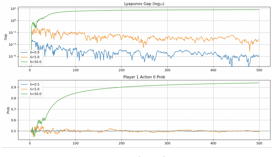
- The Jordan three-player experiments indicate that when strict diagonal dominance fails, the smoothed Frank-Wolfe dynamics lose convergence for large $\lambda$, paralleling known impossibility results for uncoupled gradient dynamics; this suggests Assumption 2.2 is close to necessary, though the paper does not prove a formal necessary condition.
- Since the variational-inequality analysis is written for polytopal strategy spaces, the same machinery should transfer to polymatrix or coupling-constrained games; a natural next test is whether the smoothed gap retains its negative drift when $\Delta(A_i)$ is replaced by a general polytope with a Bregman distance.
Editorial analysis
A structured set of objections, weighed in public.
Referee Report
Summary. The paper introduces Generalized Quantal Response Equilibrium (GQRE), a generalized quantal response solution concept based on agent-specific strongly convex penalties, and shows existence, uniqueness under diagonal dominance, and a variational inequality characterization. It proposes a decentralized smoothed Frank–Wolfe algorithm with bandit feedback from a simulator oracle and proves a finite-time bound on a smoothed gap function (Theorem 3.1). Numerical experiments compare the method against several baselines on strongly monotone and low-rank games.
Significance. If the convergence claim were fully established, the paper would offer a useful contribution: a programmable framework for solution concepts with bounded rationality, a decentralized algorithm that works with noisy bandit feedback rather than exact gradients, and a finite-time analysis of a non-standard smoothed Frank–Wolfe scheme. The VI-based verification result (Lemma 2.2) and the simulation oracle treatment are also concrete and potentially reusable. The main obstacle is that the proved object, convergence of V(π_T) to zero, is not equivalent to convergence to the unique GQRE; the gap function is not a valid distance certificate on the closure of the algorithm's domain. Because the paper's central claim is exactly that Algorithm 1 'computes the GQRE,' this issue is load-bearing.
major comments (3)
- [Appendix B and Theorem 3.1] The assertion in Appendix B that 'the issue of the gap function being zero at pure strategy profiles doesn't cause trouble' is unsupported and is load-bearing for the main theorem. Lemma A.1 establishes that V is C-smooth, hence continuous, and V vanishes at every pure strategy profile. The algorithm's iterates are constrained to Δ(A_i, ε_t) with ε_t → 0, so they may approach pure profiles. Consequently, the conclusion lim_{T→∞} V(π(T)) = 0 in probability does not imply that π(T) converges to the unique GQRE; a sequence of iterates could approach a pure non-GQRE profile while V tends to zero. The drift inequality in the proof contains no term that penalizes approach to the boundary, so it does not rule this out. To sustain the claimed convergence to GQRE, the authors must either prove that pure non-GQRE profiles cannot be limit points of Algorithm 1, or replace V with a certificate that is positive on all non-GQRE profiles in the closure of the domain, or explicitly restate the theorem as convergence to the zero set of V rather than to the GQRE.
- [Appendix A, Lemma A.1] The proof of C-smoothness of V is a sketch that does not provide the ingredients needed for the drift argument. The bound ∥∇V(π_1) − ∇V(π_2)∥ ≤ C∥π_1 − π_2∥ uses constants α_V, α_H, α_s, and c_0 that are not defined, and the claim that λ(π) is Lipschitz is stated as 'easily shown' without a derivation. Since the quadratic upper bound in equation (16) is used to control V(π(t+1)) − V(π(t)), the missing Lipschitz verification is part of the proof of Theorem 3.1. This section needs to be completed with explicit constants in terms of the game data and Assumptions 2.1–2.2.
- [Appendix B, gap positivity proof] The second-order expansion of the KL divergence near π_1 has an incorrect sign: for π̃_1(δ) = π_1 + δ(s_1 − π_1), the KL divergence is approximately (δ²/2) Σ_a (s_{1,a} − π_{1,a})² / π_{1,a}, not a negative quantity as written. The subsequent inequality '⟨·⟩ − ηKL ≈ δϵ − δ²η Σ ...' therefore does not follow as written. The conclusion that V_1(π) > 0 for small δ can still be recovered with a correct expansion because the linear term dominates for sufficiently small δ, but the proof needs correction.
minor comments (5)
- [Section 1] The phrase 'smoothened Franke-Wolfe' contains a typo; it should be 'Frank–Wolfe'.
- [Theorem 3.1 and Appendix A] The theorem is called a 'no-regret guarantee,' but R(T) is the expected value of the gap function, not a regret with respect to a comparator sequence; the terminology should be clarified.
- [Section 3, after Algorithm 1] The claimed 'efficiency' should be qualified by the simulator sample complexity: with γ_t = 1/(t+1) and ε_t = 1/((t+1) max_i |A_i|), the choice M_t = ⌈1/(ε_t γ_t²)⌉ gives cumulative simulator uses of order Ω(T⁴), which is polynomial but very large for practical T.
- [Appendix B, first paragraph] The notation in the statement 'the gradient of KL(π̃|π_i) is 0 at π̃ = π_i' is informal; it should state that the first-order term in the KL divergence vanishes at that point, which is the actual argument being used.
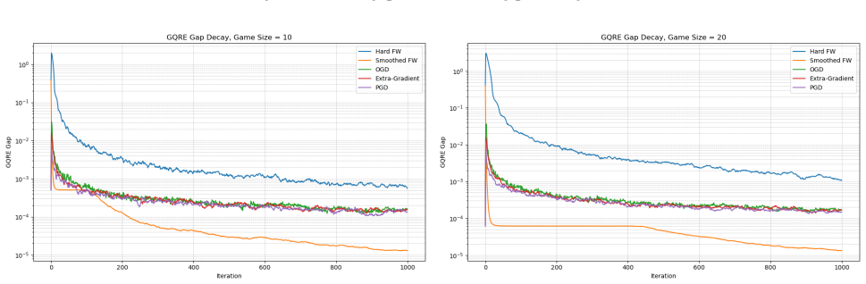
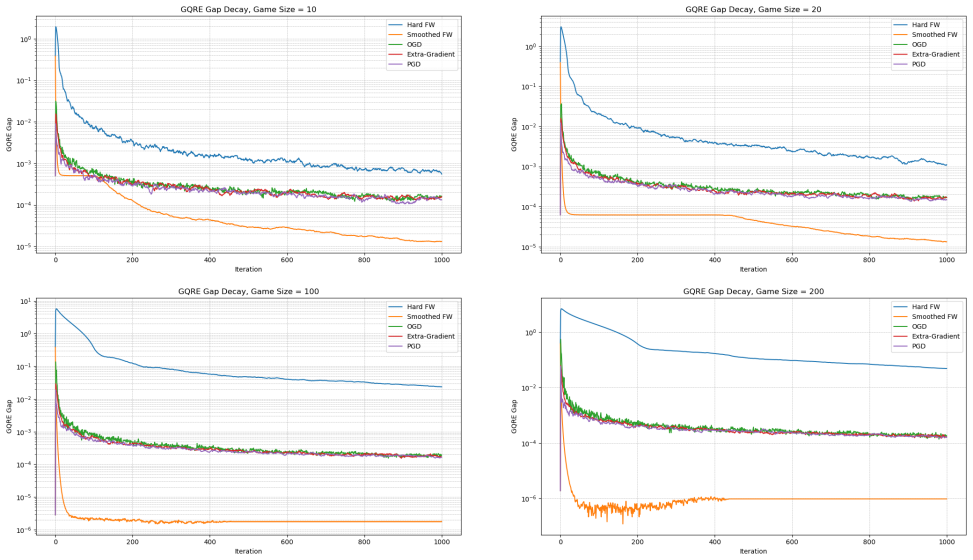
- [Section 4] The experimental comparison reports averages over 20 runs but gives no error bars or variance information, making it difficult to assess the claim of 'much more stable' performance.
Circularity Check
No significant circularity: the central convergence theorem is proved from stated assumptions; the pure-profile caveat is an unsupported step but not a circular reduction.
full rationale
The convergence theorem is not circular. Under Assumptions 2.1 and 2.2, the proof of Theorem 3.1 establishes a negative drift inequality E[V(pi_{t+1})|pi_t] <= (1-gamma_t)V(pi_t) + C4 gamma_t^2 + C5 gamma_t epsilon_t, then telescopes with gamma_t=1/(t+1), epsilon_t proportional to gamma_t, and M_t=ceil(1/(epsilon_t gamma_t^2)) to obtain R(T) <= C7/T + C6 log(T)/T. The gap function V is used only as a Lyapunov certificate; it is not fitted to the target equilibrium, and the constants are not tuned to force the conclusion. Uniqueness is imported from Rosen (1965) via Assumption 2.2, which is an external condition rather than a self-citation. The equivalence in Theorem 2.1 is a restatement of Definition 2.2 as best response in the perturbed game, used to connect to Rosen; this is an immediate characterization, not a circular prediction. The paper does contain an unresolved limitation that the skeptic correctly identifies, but it is a correctness gap rather than circularity: Appendix B proves V(pi)>0 only for full-support non-GQRE pi, and then asserts 'our gap function is 0 for all pure strategy profiles... the issue of the gap function being zero at pure strategy profiles doesn't cause trouble.' Since epsilon_t tends to 0, iterates may approach pure profiles, and V is continuous, so V -> 0 does not by itself certify convergence to the GQRE. This undermines the interpretation of Theorem 3.1 but does not make the derivation equal to its own inputs.
Assumptions & free parameters
free parameters (1)
- η (smoothing temperature)
assumptions (5)
- domain assumption Assumption 2.1: perturbed utility gradients are Lipschitz and have Lipschitz Jacobian.
- domain assumption Assumption 2.2: strict diagonal dominance, H(π)+H^T(π) negative definite for all π.
- domain assumption The unique equilibrium is fully mixed.
- standard math Donsker-Varadhan variational formula and convexity of KL divergence.
- standard math Rosen's existence theorem for concave games and Berge's theorem of the maximum.
Cite this review
Pith. "Pith review of Efficient Decentralized Learning of Generalized Quantal Response Equilibrium." pith.science (2026). https://pith.science/paper/5JJ7ZM4G
@misc{pith2026250709928,
  author       = {Pith},
  title        = {Pith review of: Efficient Decentralized Learning of Generalized Quantal Response Equilibrium},
  year         = {2026},
  howpublished = {\url{https://pith.science/paper/5JJ7ZM4G}},
  note         = {Machine review of arXiv:2507.09928}
}
read the original abstract
We study a solution concept for bounded rational agents in finite normal-form general-sum games called Generalized Quantal Response Equilibrium (GQRE) which generalizes Quantal Response Equilibrium~\citep{mckelvey1995quantal}. In our setup, each player can individually maximize a smooth, regularized expected utility of the mixed profiles used, reflecting both bounded rationality that subsumes stochastic choice and also individual choice of behaviors. After establishing existence under mild conditions, we present a computationally efficient no-regret decentralized learning algorithm via a smoothened version of the Frank--Wolfe algorithm. Our algorithm uses noisy gradient estimates via bandit-feedback from a simulation oracle that reports on repeated plays of the game. We analyze finite-time convergence properties of our algorithm under assumptions that ensure uniqueness of equilibrium, using a novel class of gap functions that generalize the Nash gap. We end by demonstrating the effectiveness of our method on a set of complex general-sum games such as high-rank two-player games, large action two-player games, and known examples of difficult multi-player games.
Figures


Figures from the paper (6 more)


Reference graph
Works this paper leans on
-
[1]
P., De Palma, A., and Thisse, J.-F
Anderson, S. P., De Palma, A., and Thisse, J.-F. (1992). Discrete choice theory of product differentiation . MIT press
work page 1992
-
[2]
Cai, Y., Oikonomou, A., and Zheng, W. (2022). Finite-time last-iterate convergence for learning in multi-player games. Advances in Neural Information Processing Systems , 35:33904--33919
work page 2022
-
[3]
Chen, Z., Ma, S., and Zhou, Y. (2022). Sample efficient stochastic policy extragradient algorithm for zero-sum markov game. In International Conference on Learning Representation
work page 2022
-
[4]
Facchinei, F. and Pang, J.-S. (2003). Finite-dimensional variational inequalities and complementarity problems . Springer
work page 2003
-
[5]
Frank, M., Wolfe, P., et al. (1956). An algorithm for quadratic programming. Naval research logistics quarterly , 3(1-2):95--110
work page 1956
-
[6]
and Levine, D
Fudenberg, D. and Levine, D. K. (1998). The theory of learning in games , volume 2. MIT press
1998
-
[7]
Gao, B. and Pavel, L. (2017). On the properties of the softmax function with application in game theory and reinforcement learning. arXiv preprint arXiv:1704.00805
arXiv 2017
-
[8]
Goeree, J. K. and Holt, C. A. (2001). Ten little treasures of game theory and ten intuitive contradictions. American Economic Review , 91(5):1402--1422
work page 2001
Show all 25 references
-
[9]
K., Holt, C
Goeree, J. K., Holt, C. A., and Palfrey, T. R. (2003). Risk averse behavior in generalized matching pennies games. Games and Economic Behavior , 45(1):97--113
2003
-
[10]
K., Holt, C
Goeree, J. K., Holt, C. A., and Palfrey, T. R. (2005). Regular quantal response equilibrium. Experimental economics , 8:347--367
2005
-
[11]
and Ta s kesen, B
Gui, Y. and Ta s kesen, B. (2025). Statistical equilibrium of optimistic beliefs. arXiv preprint arXiv:2502.09569
2025
-
[12]
A., Horta c su, A., and Kosenok, G
Haile, P. A., Horta c su, A., and Kosenok, G. (2008). On the empirical content of quantal response equilibrium. American Economic Review , 98(1):180--200
2008
-
[13]
and Sandholm, W
Hofbauer, J. and Sandholm, W. H. (2002). On the global convergence of stochastic fictitious play. Econometrica , 70(6):2265--2294
2002
-
[14]
Jordan, M., Lin, T., and Zhou, Z. (2024). Adaptive, doubly optimal no-regret learning in strongly monotone and exp-concave games with gradient feedback. Operations Research
2024
-
[15]
Juditsky, A., Nemirovski, A., and Tauvel, C. (2011). Solving variational inequalities with stochastic mirror-prox algorithm. Stochastic Systems , 1(1):17--58
2011
-
[16]
and Theobald, T
Kannan, R. and Theobald, T. (2010). Games of fixed rank: A hierarchy of bimatrix games. Economic Theory , 42:157--173
2010
-
[17]
Mazumdar, E., Panaganti, K., and Shi, L. (2024). Tractable equilibrium computation in markov games through risk aversion. arXiv preprint arXiv:2406.14156
2024 arXiv
-
[18]
McKelvey, R. D. and Palfrey, T. R. (1995). Quantal response equilibria for normal form games. Games and economic behavior , 10(1):6--38
1995
-
[19]
Melo, E. (2022). On the uniqueness of quantal response equilibria and its application to network games. Economic Theory , 74(3):681--725
2022
-
[20]
and Zhou, Z
Mertikopoulos, P. and Zhou, Z. (2019). Learning in games with continuous action sets and unknown payoff functions. Mathematical Programming , 173:465--507
2019
-
[21]
Nemirovski, A. (2004). Prox-method with rate of convergence o (1/t) for variational inequalities with lipschitz continuous monotone operators and smooth convex-concave saddle point problems. SIAM Journal on Optimization , 15(1):229--251
2004
-
[22]
Nemirovski, A., Juditsky, A., Lan, G., and Shapiro, A. (2009). Robust stochastic approximation approach to stochastic programming. SIAM Journal on optimization , 19(4):1574--1609
2009
-
[23]
Rosen, J. B. (1965). Existence and uniqueness of equilibrium points for concave n-person games. Econometrica: Journal of the Econometric Society , pages 520--534
1965
-
[24]
Selfridge, O. G. (1989). Adaptive strategies of learning a study of two-person zero-sum competition. In Proceedings of the sixth international workshop on Machine learning , pages 412--415. Elsevier
1989
-
[25]
van Damme, E. E. C. (1982). Refining the equilibrium concept for bimatrix games via control costs
1982
Reviewed August 6, 2026 · model on record in the stance chip above.
Discussion (0). Continue with ORCID to comment.