REVIEW 5 major objections 7 minor 55 references
Wavelet-Enhanced Neural ODE and Graph Attention for Interpretable Energy Forecasting
T0 review · 5 major / 7 minor · reviewed 2026-08-06 · deepseek-v4-flash
Pith's one-line read A hybrid neural network that fuses Neural ODEs, graph attention, and wavelet transforms reports state-of-the-art forecasting accuracy across seven energy datasets, with SHAP-based interpretability.
desk verdict A reasonable multi-path fusion idea is undermined by internally inconsistent reported metrics and a lopsided baseline comparison, so the central claim does not stand. read the letter →
The pith
A machine-rendered reading of the paper's core claim, the machinery that carries it, and where it could break.
The reading
What carries the argument
The load-bearing mechanism is a multi-path fusion pipeline: a Neural ODE with graph attention (state dynamics $dh/dt = f_\theta(h, A)$ using a dynamic adjacency matrix $A$ built from thresholded Pearson correlations, solved by one RK4 step), a Daubechies-inspired 1D convolution with global average pooling, a parametric transform using learnable frequency, amplitude, and phase, and a direct dense path. The concatenated feature vector is refined by dense layers with dropout and a residual connection, and the entire model is trained on mean squared error with Bayesian hyperparameter tuning and early stopping. What this machinery is doing is letting the model simultaneously represent continuous temporal dynamics, feature interdependencies, multi-scale transients, and periodic patterns, then merge them into a single scalar prediction.
What would settle it
Re-run the benchmark with the adjacency matrix computed only from the training portion, hand the same 51 engineered features to N-BEATS, N-HiTS, and TCN, and tune them with the same hyperparameter budget; if their RMSE and MAE approach or beat the reported values on ETTh1 and ETTm1, the claimed consistency would be an artifact of the evaluation setup.
Extended reading notes
Core claim
The central claim is that fusing four parallel feature-extraction paths — a Neural ODE path with graph attention, a Daubechies-inspired wavelet convolution path, a learnable parametric frequency path, and a direct dense path — produces a forecaster that outperforms established baselines across diverse energy datasets. The adjacency matrix for the graph attention is built from thresholded Pearson correlations among features, allowing the model to learn inter-feature dependencies directly from data. The ODE state is evolved with a single fourth-order Runge-Kutta step at dt = 0.01, and all paths are concatenated and refined through dense layers with dropout and a residual connection. On the ETT datasets the model reports the best RMSE and MAE in 22 of 23 windowed settings, and on Waste and Hydro it achieves R-squared values above 0.98. The paper also argues through an ablation study that each path contributes, with the full model reaching R-squared 0.9606 on ETTh1 versus 0.7447 for the ODE-only configuration.
Load-bearing premise
The reported margin of improvement depends on the baselines being given the same engineered inputs, the same data split, and comparable tuning effort, but the paper does not document that, and the correlation graph is built on the full dataset before the train/test split.
Editorial extensions
If this is right
- If the reported results are reproducible, the architecture offers a single model that works across hourly, 15-minute, and monthly energy data without changing its core design.
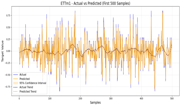
- The claimed margins on ETT datasets — for example MSE of 0.0135 on ETTh1 versus 0.2970 for the best baseline — would make the model a new benchmark for transformer-temperature forecasting.
- The ablation study indicates that removing any path degrades accuracy, with the ODE-only version performing far worse, which suggests the multi-path fusion itself is the source of the reported gains.
- SHAP analysis points to a small set of features — oil-temperature differences and lags on ETT data, rolling means and lags on renewable data — that could guide cheaper feature engineering in practical deployments.
- The paper's own Solar results, where a simple attention model beats the proposed model on RMSE, R-squared, and MAE, imply the architecture does not yet handle irregular high-variance renewable patterns as well as it handles smoother series.
Reading between the lines
- A direct extension the paper leaves implicit: recompute the adjacency matrix from sliding windows or learn it end-to-end, since the static full-series correlation used here cannot adapt to regime shifts in energy data.
- The single RK4 step with a fixed tiny dt makes the continuous-time claim largely symbolic; a meaningful test would feed irregular timestamps and allow variable integration steps to see whether the ODE path actually buys accuracy for unevenly sampled sensors.
- The claimed state-of-the-art status would be much stronger if tested against modern transformer-based forecasters such as PatchTST, iTransformer, or TimesNet, which are absent from the baseline set.
- The SHAP analysis is applied to engineered features rather than raw sensor channels, so its practical value depends on whether those engineered features are available at deployment time; otherwise the interpretability finding would not transfer to operational settings.
Editorial analysis
A structured set of objections, weighed in public.
Referee Report
Summary. The paper proposes a hybrid time-series forecasting architecture that combines a Neural ODE (solved by one RK4 step with dt=0.01), graph attention over a Pearson-correlation adjacency matrix, a learnable 'Daubechies-inspired' convolution path, a parametric frequency transform, and a dense path, with SHAP used for interpretability. The model is evaluated on four ETT datasets and three monthly EIA energy datasets against baselines such as N-BEATS, N-HiTS, TCN, XGBoost, RandomForest, LSTM-Attention, and Informer. The paper claims consistent state-of-the-art performance, reports an ablation study on ETTh1, and provides execution-time, memory, and SHAP analyses.
Significance. If the reported results were reliable, the architecture would be a useful contribution to energy time-series forecasting, and the paper does provide a detailed architecture description, complexity analysis, and SHAP-based feature interpretation. However, the evaluation is the load-bearing part of the claim, and it is not internally consistent: the ablation table contains metric values that cannot be reconciled, the correlation-based graph is built on the full dataset before the train/test split, and the baseline comparison is lopsided and omits current state-of-the-art methods. These problems mean that the central claim of consistent superiority is not supported by the manuscript as written.
major comments (5)
- [Section 8, Tables 9 and 10] The ablation table is internally inconsistent, so the paper's own numbers undermine the conclusion that each architectural component contributes. In Table 9, the Full Model reports MSE=0.0135 and RMSE=0.1161, which are consistent (0.1161^2=0.0135), but the other rows are not: No ODE has MSE=0.0143 and RMSE=0.1155, whose square is 0.0133; No Daubechies has MSE=0.0172 and RMSE=0.1059, whose square is 0.0112; No Dense has MSE=0.0268 and RMSE=0.1827, whose square is 0.0334. Additionally, for the Full Model, Table 8 reports ME=0.0498 and SDE=0.1416, which would imply RMSE=sqrt(ME^2+SDE^2)=0.150, not the 0.1161 reported in Table 9. These discrepancies are far too large to be rounding artifacts, and since the ablation is the primary evidence for the contribution of each path, the evaluation cannot be regarded as valid.
- [Section 2.2, Eq. (1), and Section 5] The adjacency matrix A is computed from Pearson correlations over the full dataset X before the 80/20 train/test split described in Section 5. Algorithm 1, line 1, repeats this full-data computation. This means that test-set information is used to construct the graph that guides the attention mechanism during training and evaluation, which is a form of test leakage. A valid protocol would estimate the correlations and threshold on the training portion only, or use a rolling-window graph, and then freeze A before scoring the test set. As written, the reported margins may be inflated by this leakage.
- [Section 5.1 and Section 6, Tables 2 and 3] The claim that the proposed model 'consistently outperforms state-of-the-art baselines' is not supported by the baseline selection or by the feature-setting symmetry. For the ETT datasets, N-BEATS, N-HiTS, and TCN are not current state-of-the-art; well-known stronger baselines such as PatchTST, iTransformer, TimesNet, and DLinear are absent. More importantly, the paper does not state whether those baselines received the 51 engineered features that the proposed model uses, or only raw windows. The hyperparameter description in Section 5.2 for the Darts models (input chunk length, layer widths, number of filters) suggests they do not receive the same engineered features. If the baselines were not given the same inputs, the comparison is not on the same forecasting task, and the large error gaps reported in Tables 2 and 3 are not meaningful.
- [Section 6.1.1, Tables 4 and 5] The paper's summary claim of consistent wins is contradicted by its own Table 4. The text in Section 6.1.1 states that for the Solar dataset the Attention-based model outperforms the proposed model in RMSE, R2, and MAE (7.2984 vs 7.8372, 0.8886 vs 0.8716, and 5.4474 vs 5.4902). Yet Table 5 reports that the proposed model wins 22 of 23 RMSE settings and 22 of 23 MAE settings. If the Solar result is included in those counts, the table is wrong; if it is excluded, the counting basis is not stated. Either way, the 'consistently outperforms' claim in the abstract and Section 6 is not supported by the paper's own results.
- [Section 2.3, Eq. (2)-(7)] The Neural ODE path as implemented performs a single RK4 step with dt=0.01 from the projected input, which is equivalent to a fixed residual update rather than an integration over a continuous interval. The text further claims that the framework can evaluate the state at arbitrary time points for irregularly sampled data, but no experiment or procedure demonstrates this capability. The contribution would be better framed as a residual-style ODE-inspired block than as a continuous-time model, and the claim of flexible handling of irregular sampling should be removed unless it is actually exercised and tested.
minor comments (7)
- [Abstract] The abstract contains grammar errors, including 'This paper introduce' instead of 'This paper introduces', and 'proving its robustness' should be softened to 'demonstrating robustness' or similar. Please proofread the entire text.
- [Section 2.5, Eq. (10)] The concatenated feature dimension is h + h/2 + h/2 + h/4 = 2.25h, not 'approximately 2h' as stated; the text should either correct the formula or the stated total.
- [Figure 3] Figure 3 is captioned 'Adams-Bashforth ODE Solver Workflow' and shows Euler and Adams-Bashforth equations, but the text refers to Figure 3 as the proposed Neural ODE with graph attention and RK4. The figure and caption do not match the described architecture.
- [Table 3] The ETTm2 rows for N-BEATS, N-HiTS, and TCN are identical to the corresponding ETTh1 rows for windows 96, 120, 336, and 720 (e.g., ETTm2 Window 96 N-BEATS RMSE=0.6334, MAE=0.4962, exactly as ETTh1 Window 96). This looks like a copy-paste error and should be corrected.
- [Table 6] The Solar non-windowed hyperparameter row lists only four values ('96, 8, 63, 0.0001') whereas other rows list five; the dropout rate is missing and should be specified.
- [Section 2.4.2] Calling the learnable Conv1D path a 'Daubechies transform' is misleading because the kernel is learned and not constrained to a Daubechies wavelet basis; the text should consistently say 'wavelet-inspired convolutional path' to avoid overclaiming.
- [References] References [34] and [52] are duplicates of the same Informer paper; please merge them and cite the published version.
Circularity Check
No circular derivation: the model is empirical and no prediction reduces to a fitted input or self-citation; the noted issues are evaluation-integrity concerns, not circularity.
full rationale
This is an empirical forecasting paper: the proposed multi-path network is trained to minimize MSE and evaluated on held-out test metrics, with no derived constants, no fitted parameter later renamed as a prediction, and no load-bearing self-citation or imported uniqueness theorem that would force a particular architectural choice. The graph-construction step in Eq. (1) is computed on the full dataset X before the 80/20 split described in Section 5, and Section 8's Table 9 is internally inconsistent with the definitional identity RMSE = sqrt(MSE) (e.g., Full Model MSE=0.0135/RMSE=0.1161 is consistent, but No ODE MSE=0.0143/RMSE=0.1155 and No Daubechies MSE=0.0172/RMSE=0.1059 are not), so the reported ablation and claim of consistent state-of-the-art performance are not reliable as stated. These are serious benchmark-integrity and internal-consistency problems, but they are not cases where a claimed prediction or first-principles result is equivalent to its inputs by construction, nor do the model's equations reduce to a self-citation chain. Accordingly, no circularity step is identified.
Assumptions & free parameters
free parameters (6)
- Correlation threshold tau =
0.3
- RK4 step size dt =
0.01
- Per-dataset hidden dimension h =
Varies per dataset, e.g., 64, 128, 48, 446, 96 in Table 6
- Per-dataset dropout rate, learning rate, batch size, epochs =
Varies per dataset, e.g., dropout 0.1-0.5, lr 1e-4 to 1e-2
- Number of features after RFE =
8
- Feature engineering window sizes and lag sets =
EIA: window 3, lags 1-6; ETT: windows 5/10/20, lags 1-28
assumptions (5)
- domain assumption The future target value is a function of the engineered feature vector, so a feedforward network on lags, rolling statistics, and calendar features suffices for forecasting.
- ad hoc to paper A thresholded Pearson correlation matrix computed on the full dataset is a valid graph structure for feature interactions and does not leak test information.
- ad hoc to paper One RK4 step with dt=0.01 captures the continuous-time dynamics needed for forecasting.
- ad hoc to paper A learnable Conv1D with random initialization behaves like a Daubechies wavelet transform.
- domain assumption The 80/20 data split preserves temporal order and avoids lookahead in lag and rolling features.
Cite this review
Pith. "Pith review of Wavelet-Enhanced Neural ODE and Graph Attention for Interpretable Energy Forecasting." pith.science (2026). https://pith.science/paper/W5EVSBHQ
@misc{pith2026250710132,
  author       = {Pith},
  title        = {Pith review of: Wavelet-Enhanced Neural ODE and Graph Attention for Interpretable Energy Forecasting},
  year         = {2026},
  howpublished = {\url{https://pith.science/paper/W5EVSBHQ}},
  note         = {Machine review of arXiv:2507.10132}
}
read the original abstract
Accurate forecasting of energy demand and supply is critical for optimizing sustainable energy systems, yet it is challenged by the variability of renewable sources and dynamic consumption patterns. This paper introduces a neural framework that integrates continuous-time Neural Ordinary Differential Equations (Neural ODEs), graph attention, multi-resolution wavelet transformations, and adaptive learning of frequencies to address the issues of time series prediction. The model employs a robust ODE solver, using the Runge-Kutta method, paired with graph-based attention and residual connections to better understand both structural and temporal patterns. Through wavelet-based feature extraction and adaptive frequency modulation, it adeptly captures and models diverse, multi-scale temporal dynamics. When evaluated across seven diverse datasets: ETTh1, ETTh2, ETTm1, ETTm2 (electricity transformer temperature), and Waste, Solar, and Hydro (renewable energy), this architecture consistently outperforms state-of-the-art baselines in various forecasting metrics, proving its robustness in capturing complex temporal dependencies. Furthermore, the model enhances interpretability through SHAP analysis, making it suitable for sustainable energy applications.
Figures


Figures from the paper (24 more)




Reference graph
Works this paper leans on
-
[1]
Z. Chen, M. Ma, T. Li, H. Wang, C. Li, Long sequence time-series forecasting with deep learning: A survey, Information Fusion 97 (2023) 101819. doi:https://doi.org/10.1016/j.inffus.2023.101819. URL https://www.sciencedirect.com/science/article/pii/S1566253523001355
arXiv 2023
-
[2]
R. T. Chen, Y . Rubanova, J. Bettencourt, D. K. Duvenaud, Neural ordinary di fferential equations, Advances in Neural Information Processing Systems 31 (2018) 6571–6583
work page 2018
-
[3]
Y . Rubanova, R. T. Chen, D. K. Duvenaud, Latent ordinary di fferential equations for irregularly-sampled time series, Advances in Neural Information Processing Systems 32 (2019) 5320–5330
work page 2019
- [4]
-
[5]
S. Massaroli, M. Poli, J. Park, A. Yamashita, H. Asama, Stable neural flows, Advances in Neural Information Processing Systems 35 (2022) 12556–12569
work page 2022
-
[6]
A. Sholokhov, Y . Liu, H. Mansour, S. Nabi, Physics-informed neural ode (pinode): embedding physics into models using collocation points, Scientific Reports 13 (1) (2023) 10166
work page 2023
-
[7]
G. Woo, C. Liu, D. Sahoo, A. Kumar, S. Hoi, CoST: Contrastive learning of disentangled seasonal-trend represen- tations for time series forecasting, in: International Conference on Learning Representations, 2022, p. –. URL https://openreview.net/forum?id=PilZY3omXV2
work page 2022
-
[8]
J. Moon, S. Rho, S. W. Baik, Toward explainable electrical load forecasting of buildings: A comparative study of tree-based ensemble methods with shapley values, Sustainable Energy Technologies and Assessments 54 (2022) 102888
work page 2022
Show all 55 references
-
[9]
X. Luo, D. Zhang, An adaptive deep learning framework for day-ahead forecasting of photovoltaic power genera- tion, Sustainable Energy Technologies and Assessments 52 (2022) 102326
2022
-
[10]
W. Ma, W. Wu, S. F. Ahmed, G. Liu, Techno-economic feasibility of utilizing electrical load forecasting in micro- grid optimization planning, Sustainable Energy Technologies and Assessments 73 (2025) 104135
2025
-
[11]
Cobos-Maestre, M
M. Cobos-Maestre, M. Flores-Soriano, D. F. Barrero, Swan: A multihead autoregressive attention model for solar wind speed forecasting, Expert Systems with Applications 252 (2024) 124128
2024
-
[12]
Kim, T.-H
S. Kim, T.-H. Lee, J. Lee, Tmf-gnn: Temporal matrix factorization-based graph neural network for multivariate time series forecasting with missing values, Expert Systems with Applications (2025) 127001
2025
-
[13]
Gil-Gamboa, P
A. Gil-Gamboa, P. Paneque, O. Trull, A. Troncoso, Medium-term water consumption forecasting based on deep neural networks, Expert Systems with Applications 247 (2024) 123234
2024
-
[14]
Madhusudhanan, J
K. Madhusudhanan, J. Burchert, N. Duong-Trung, S. Born, L. Schmidt-Thieme, U-net inspired transformer archi- tecture for far horizon time series forecasting, in: Joint European Conference on Machine Learning and Knowledge Discovery in Databases, Springer, 2022, pp. 36–52. 40
2022
-
[15]
Saeed, S
F. Saeed, S. Aldera, Adaptive renewable energy forecasting utilizing a data-driven pca-transformer architecture, IEEE Access 12 (2024) 109269–109280. doi:10.1109/ACCESS.2024.3440226
2024
-
[16]
L. Shen, Y . Wei, Y . Wang, Gbt: Two-stage transformer framework for non-stationary time series forecasting, Neural Networks 165 (2023) 953–970. doi:https://doi.org/10.1016/j.neunet.2023.06.044. URL https://doi.org/10.1016/j.neunet.2023.06.044
2023 doi
-
[17]
M. Rhif, A. Ben Abbes, I. R. Farah, B. Mart ´ınez, Y . Sang, Wavelet transform application for /in non-stationary time-series analysis: A review, Applied Sciences 9 (7) (2019) 1345
2019
-
[18]
Q. Ma, L. Shen, W. Chen, J. Wang, J. Wei, Z. Yu, Functional echo state network for time series classification, Information Sciences 373 (2016) 1–20
2016
-
[19]
Ashwini, V
C. Ashwini, V . Sellam, Corn disease detection based on deep neural network for substantiating the crop yield, Appl Math 16 (3) (2022) 423–433
2022
-
[20]
H. H. El-Sayed, S. K. Refaay, S. A. Ali, M. T. El-Melegy, Chain based leader selection using neural network in wireless sensor networks protocols, in: 2021 9th International Japan-Africa Conference on Electronics, Communi- cations, and Computations (JAC-ECC), IEEE, 2021, pp. 105–110
2021
-
[21]
J. F. Torres, D. Hadjout, A. Sebaa, F. Mart ´ınez- ´Alvarez, A. Troncoso, Deep learning for time series forecasting: a survey, Big Data 9 (1) (2021) 3–21
2021
-
[22]
B. Lim, S. ¨O. Arık, N. Loe ff, T. Pfister, Temporal fusion transformers for interpretable multi-horizon time series forecasting, International Journal of Forecasting 37 (4) (2021) 1748–1764
2021
-
[23]
J. Gu, Z. Jia, T. Cai, X. Song, A. Mahmood, Dynamic correlation adjacency-matrix-based graph neural networks for traffic flow prediction, Sensors 23 (6) (2023). URL https://www.mdpi.com/1424-8220/23/6/2897
2023
-
[24]
D. Yao, Z. Li, B. Li, C. Zhang, H. Ma, Similarity graph-correlation reconstruction network for unsupervised cross- modal hashing, Expert Systems with Applications 237 (2024) 121516
2024
-
[25]
Y . Zeng, Z. Li, Z. Tang, Z. Chen, H. Ma, Heterogeneous graph convolution based on in-domain self-supervision for multimodal sentiment analysis, Expert Systems with Applications 213 (2023) 119240
2023
-
[26]
Y . Qin, W. Ju, H. Wu, X. Luo, M. Zhang, Learning graph ode for continuous-time sequential recommendation, IEEE Transactions on Knowledge and Data Engineering 36 (7) (2024) 3224–3236. doi:10.1109/TKDE.2024.3349397
2024
-
[27]
J. C. Butcher, A history of runge-kutta methods, Applied numerical mathematics 20 (3) (1996) 247–260
1996
-
[28]
J. Yan, L. Hu, Z. Zhen, F. Wang, G. Qiu, Y . Li, L. Yao, M. Shafie-khah, J. P. Catal˜ao, Frequency-domain decompo- sition and deep learning based solar pv power ultra-short-term forecasting model, IEEE Transactions on Industry Applications 57 (4) (2021) 3282–3295
2021
-
[29]
Olsavszky, M
V . Olsavszky, M. Dosius, C. Vladescu, J. Benecke, Time series analysis and forecasting with automated machine learning on a national icd-10 database, International journal of environmental research and public health 17 (14) (2020) 4979
2020
-
[30]
A. K. Alexandridis, A. D. Zapranis, Wavelet neural networks: A practical guide, Neural Networks 42 (2013) 1–27
2013
-
[31]
Y . Gal, Z. Ghahramani, Dropout as a bayesian approximation: Representing model uncertainty in deep learning, in: international conference on machine learning, PMLR, 2016, pp. 1050–1059
2016
-
[32]
J. Jin, J. Kim, Forecasting natural gas prices using wavelets, time series, and artificial neural networks, PLOS ONE 10 (11) (2015) 1–23. doi:10.1371/journal.pone.0142064. URL https://doi.org/10.1371/journal.pone.0142064
2015 doi
-
[33]
L. Du, R. Gao, P. N. Suganthan, D. Z. Wang, Bayesian optimization based dynamic ensemble for time series forecasting, Information Sciences 591 (2022) 155–175. doi:https://doi.org/10.1016/j.ins.2022.01.010. URL https://www.sciencedirect.com/science/article/pii/S0020025522000135
2022 doi
-
[34]
H. Zhou, S. Zhang, J. Peng, S. Zhang, J. Li, H. Xiong, W. Zhang, Informer: Beyond e fficient transformer for long sequence time-series forecasting, in: Proceedings of AAAI, 2021, p. –
2021
-
[35]
T. U. E. I. A. (EIA), U.s. energy information administration - eia - independent statistics and analysis (2024). URL https://bitly.cx/vzBi
2024
-
[36]
Chandola, A
V . Chandola, A. Banerjee, V . Kumar, Anomaly detection: A survey, ACM computing surveys (CSUR) 41 (3) (2009) 1–58
2009
-
[37]
M. N. Ramli, A. S. Yahaya, N. Ramli, N. F. F. M. Yusof, M. Abdullah, Roles of imputation methods for filling the missing values: A review, Advances in Environmental Biology 7 (12 S2) (2013) 3861–3870
2013
-
[38]
V . G. Raju, K. P. Lakshmi, V . M. Jain, A. Kalidindi, V . Padma, Study the influence of normalization/transformation process on the accuracy of supervised classification, in: 2020 Third International Conference on Smart Systems and Inventive Technology (ICSSIT), IEEE, 2020, p...
2020
-
[39]
Christ, N
M. Christ, N. Braun, J. Neu ffer, A. W. Kempa-Liehr, Time series feature extraction on basis of scalable hypothesis tests (tsfresh–a python package), Neurocomputing 307 (2018) 72–77
2018
-
[40]
Lai, W.-C
G. Lai, W.-C. Chang, Y . Yang, H. Liu, Modeling long-and short-term temporal patterns with deep neural networks, in: The 41st international ACM SIGIR conference on research & development in information retrieval, 2018, pp. 41 95–104
2018
-
[41]
Hyndman, Forecasting: principles and practice, OTexts, 2018
R. Hyndman, Forecasting: principles and practice, OTexts, 2018
2018
-
[42]
Proietti, D
T. Proietti, D. J. Pedregal, Seasonality in high frequency time series, Econometrics and Statistics 27 (2023) 62–82
2023
-
[43]
Bloomfield, Fourier analysis of time series: an introduction, John Wiley & Sons, 2004
P. Bloomfield, Fourier analysis of time series: an introduction, John Wiley & Sons, 2004
2004
-
[44]
Pavlyuk, Feature selection and extraction in spatiotemporal tra ffic forecasting: a systematic literature review, European Transport Research Review 11 (1) (2019) 6
D. Pavlyuk, Feature selection and extraction in spatiotemporal tra ffic forecasting: a systematic literature review, European Transport Research Review 11 (1) (2019) 6
2019
-
[45]
X.-w. Chen, J. C. Jeong, Enhanced recursive feature elimination, in: Sixth international conference on machine learning and applications (ICMLA 2007), IEEE, 2007, pp. 429–435
2007
-
[46]
B. N. Oreshkin, D. Carpov, N. Chapados, Y . Bengio, N-beats: Neural basis expansion analysis for interpretable time series forecasting, arXiv preprint arXiv:1905.10437 (2019)
2019 arXiv
-
[47]
Challu, K
C. Challu, K. G. Olivares, B. N. Oreshkin, F. G. Ramirez, M. M. Canseco, A. Dubrawski, Nhits: Neural hierarchical interpolation for time series forecasting, in: Proceedings of the AAAI conference on artificial intelligence, V ol. 37, 2023, pp. 6989–6997
2023
-
[48]
Hewage, A
P. Hewage, A. Behera, M. Trovati, E. Pereira, M. Ghahremani, F. Palmieri, Y . Liu, Temporal convolutional neu- ral (tcn) network for an e ffective weather forecasting using time-series data from the local weather station, Soft Computing 24 (2020) 16453–16482
2020
-
[49]
T. Chen, C. Guestrin, Xgboost: A scalable tree boosting system, in: Proceedings of the 22nd acm sigkdd interna- tional conference on knowledge discovery and data mining, 2016, pp. 785–794
2016
-
[50]
Breiman, Random forests, Machine learning 45 (2001) 5–32
L. Breiman, Random forests, Machine learning 45 (2001) 5–32
2001
-
[51]
Vaswani, N
A. Vaswani, N. Shazeer, N. Parmar, J. Uszkoreit, L. Jones, A. N. Gomez, Ł. Kaiser, I. Polosukhin, Attention is all you need, Advances in neural information processing systems 30 (2017)
2017
-
[52]
H. Zhou, S. Zhang, J. Peng, S. Zhang, J. Li, H. Xiong, W. Zhang, Informer: Beyond e fficient transformer for long sequence time-series forecasting, in: Proceedings of the AAAI conference on artificial intelligence, V ol. 35, 2021, pp. 11106–11115
2021
-
[53]
Akiba, S
T. Akiba, S. Sano, T. Yanase, T. Ohta, M. Koyama, Optuna: A next-generation hyperparameter optimization frame- work, in: Proceedings of the 25th ACM SIGKDD international conference on knowledge discovery & data mining, 2019, pp. 2623–2631
2019
-
[54]
Lundberg, A unified approach to interpreting model predictions, arXiv preprint arXiv:1705.07874 (2017)
S. Lundberg, A unified approach to interpreting model predictions, arXiv preprint arXiv:1705.07874 (2017)
2017 arXiv
-
[55]
Liang, S
Y . Liang, S. Li, C. Yan, M. Li, C. Jiang, Explaining the black-box model: A survey of local interpretation methods for deep neural networks, Neurocomputing 419 (2021) 168–182. 42
2021
Reviewed August 6, 2026 · model on record in the stance chip above.
Discussion (0). Continue with ORCID to comment.