Better Regret Rates in Bilateral Trade via Sublinear Budget Violation

Alberto Marchesi; Anna Lunghi; Matteo Castiglioni

REVIEW 3 major objections 4 minor 1 cited by

Better Regret Rates in Bilateral Trade via Sublinear Budget Violation

T0 review · 3 major / 4 minor · reviewed 2026-08-06 · deepseek-v4-flash

Challenge this review Re-run · record.json Download PDF Read on arXiv ↗ Review JSON

Pith's one-line read A regret-violation trade-off for repeated bilateral trade is proposed, but the lower bound theorem is flawed as written.

desk verdict The upper bound is a real contribution, but the matching lower bound is vacuous as stated: substituting the paper's own parameters into Theorem 5.18 gives a negative lower bound, so the claimed full characterization does not hold. read the letter →

arxiv 2507.11419 v1 pith:7RBUEM3A submitted 2025-07-15 cs.GT cs.LG

Anna Lunghi , Matteo Castiglioni , Alberto Marchesi This is my paper · ORCID

classification cs.GTcs.LG

keywords budgetbalanceregretboundviolationbetaconstraintdesign

verification ladder T0 review T1 audit T2 compute T3 formal

The pith

A machine-rendered reading of the paper's core claim, the machinery that carries it, and where it could break.

The reading

Repeated bilateral trade is a problem where a broker sets prices for a seller and a buyer each day, hoping to maximize total gain from trade. Strong budget balance, where the broker never loses money, makes low regret impossible. Earlier work introduced global budget balance, allowing losses only over the whole horizon, and achieved O~(T^{3/4}) regret with a lower bound of Ω(T^{5/7}). This paper asks what happens if the broker is allowed to violate the global budget by a controllable amount T^β. It proposes algorithms that, for β between 3/4 and 6/7, achieve regret about T^{1-β/3} while keeping violation below T^β. The upper bound uses an adaptive grid of price pairs close to the diagonal and a sleeping-experts subroutine for the adversarial case.

The paper also claims a matching lower bound, constructed with two copies of an apple-tasting gadget. However, the lower bound theorem as printed is problematic. The theorem states RT ≥ min{ (1/2048) N ϵ^2 - 3gT^β, (3/32) ϵT - 3gT^β }, but the proof's second case actually yields a term proportional to N/ϵ^2, not Nϵ^2. Substituting the paper's own parameters (g = T^{1-4β/3}/24, N = T^{1-β}/200) gives a negative lower bound for the endpoints β=3/4 and β=6/7, meaning the claimed Ω(T^{1-β/3}) does not follow. This appears to be a fixable typo rather than a conceptual impossibility, but until corrected, the full characterization is not supported.

Extended reading notes

Core claim

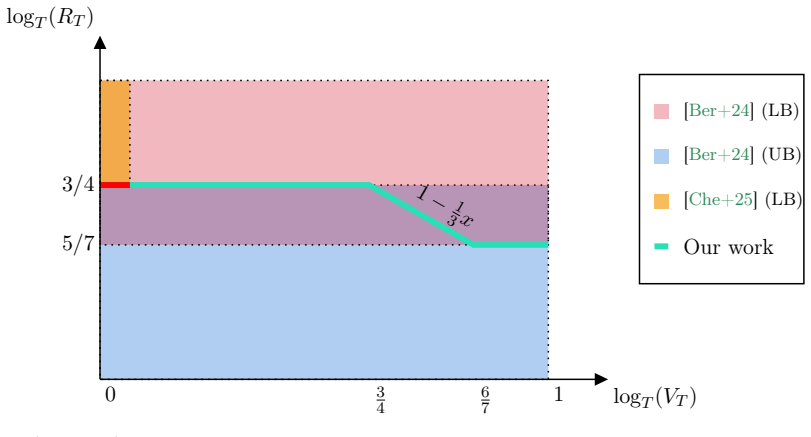
The paper's central claim is Theorem 1.1 and Theorem 1.2: for any β in [3/4, 6/7], there is an algorithm with VT ≤ O~(T^β) and RT ≤ O~(T^{1-β/3}) against adversarial valuations, and any algorithm with VT ≤ T^β must suffer RT ≥ Ω(T^{1-β/3}) even under stochastic valuations with two-bit feedback. If correct, this fully characterizes the regret-violation trade-off and shows the prior bounds of Bernasconi et al. are tight.

Load-bearing premise

The lower bound construction in Section 5 assumes that playing in the exploration region N_k is the only way to distinguish the k-th perturbed instance from the base instance, and that the KL divergence of the feedback distributions is at most O(ϵ^2/γ6) (Lemma 5.16). The proof then relies on this to relate exploration counts to regret across instances. If this KL bound is too loose, or if the revenue of points outside the exploration/exploitation grid can effectively compensate violations (Lemmas 5.7-5.9 fail), the claimed Ω(T^{1-β/3}) lower bound cannot hold.

Share X Bluesky LinkedIn Reddit HN

Signed reviews

No signed human review yet.

Editorial analysis

A structured set of objections, weighed in public.

Desk editor's note, referee report, and a circularity audit.

Desk Editor's Note

read the letter

The paper has one solid result and one broken one. The solid result is the upper bound: an adaptive-grid algorithm that, with budget violation T^β, achieves regret O~(T^{1−β/3}) for adversarial valuations with one-bit feedback. The dynamic-regret bound for sleeping experts and the runtime construction of the grid are genuinely new, and the special cases recover the known O~(T^{3/4}) and O~(T^{5/7}) rates. I believe the upper-bound analysis is basically correct, modulo fixable typos (e.g., α in Algorithm 5 should be T^{β/3}, not T^{1/3}). That part is worth publishing on its own.

The lower bound is the problem. Theorem 5.18 claims R_T ≥ min{ N/(2048ε²) − 3gT^β, 3εT/32 − 3gT^β }. With the paper's own parameters (g = T^{1−4β/3}/24, N = T^{1−β}/200, ε = g/(12(N+1))), both arguments are negative for every β ∈ [3/4, 6/7]: the εT term is about 0.065·T^{1−β/3}, while 3gT^β is 0.125·T^{1−β/3}. So the theorem is vacuous. This is not just a typo in the theorem statement. The proof's second case derives a different expression (with a γ6/(512ε²) factor), and even with the best possible constant the violation term swamps the regret term because ε and g are tied: ε ≈ g/N, making εT and gT^β the same order of T^{1−β/3}. The construction as parameterized cannot yield a positive lower bound. This is a load-bearing failure: Theorem 1.2 and the abstract's claim of a full characterization collapse. The lower-bound section also has smaller inconsistencies (e.g., the N/ε² vs N/ε² sign issues in Lemma 5.16 and the confusion between N as the number of instances and the parameter in Section 5.1).

The paper is not a waste of time. The upper-bound technique is clever and the authors engage honestly with prior work. But the main advertised result is unproven. If the lower bound can be repaired by changing the construction or the parameters, the paper could be strong; if not, the authors should publish the upper bound alone and drop the characterization claim. A serious editor should send this to peer review, because the upper bound is substantial and the lower-bound failure is the kind of thing a careful referee might catch and the authors can fix. My recommendation: reject the current version, but invite a revision that either fixes the lower bound or states the result as an upper bound only.

Referee Report

3 major / 4 minor

Summary. The paper studies repeated bilateral trade when the learner is allowed to violate the global budget-balance constraint by at most T^β over T rounds. For β in [3/4, 6/7], it proposes a stochastic-setting algorithm (Section 3) and an adversarial-setting algorithm (Section 4) achieving regret O~(T^{1−β/3}) with violation O~(T^β), and claims a matching lower bound Ω(T^{1−β/3}) in Section 5. If correct, this would fully characterize the regret–violation trade-off and would close the gaps left by Bernasconi et al. [Ber+24] and Chen et al. [Che+25].

Significance. The upper-bound part of the paper is technically substantive: the adaptive-grid construction, the unbiased GFT estimator for non-SBB mechanisms, and the sleeping-experts dynamic regret bound are interesting and appear internally coherent. The claimed lower bound, however, is the load-bearing component that would turn the paper into a full characterization. As discussed below, Theorem 5.18, on which Theorem 1.2 rests, is vacuous under the paper's own parameter choices. Since the advertised main contribution is the matching lower bound and the resulting full characterization, the paper's central claim is not established by the given proof.

major comments (3)

[§5.6, Theorem 5.18] The stated lower bound is vacuous under the parameters defined in §5.1. With N = (1/200)T^{1−β}, g = (1/24)T^{1−4β/3}, and ε = g/(12(N+1)) ≈ (25/36)T^{−β/3}, the second argument of the min in Theorem 5.18 equals (3/32)εT − 3gT^β = ((25/384) − (1/8))T^{1−β/3} = −(23/384)T^{1−β/3} < 0 for every β ∈ [3/4, 6/7]. The first argument, (1/2048)N/ε² − 3gT^β, is also negative because (1/2048)N/ε² ≈ 0.0005·T^{1−β/3}, which is smaller than 0.125·T^{1−β/3}. A lower bound of the form RT ≥ (negative quantity) is true for all algorithms and cannot imply the claimed Ω(T^{1−β/3}). This invalidates Theorem 1.2, the matching lower bound advertised in the abstract and introduction.
[§5.6, proof of Theorem 5.18] The proof's second case derives R0_T ≥ (1/32)·γ6·(N−1)·(1/(4ε))² − 3gT^β, which with γ6 ≥ 1/16 evaluates to at least (N−1)/(8192ε²) − 3gT^β. This does not match the displayed first argument of the min in the theorem statement, (1/2048)N/ε² − 3gT^β; the factor-four discrepancy cannot be absorbed by γ6, whose lower bound is 1/16. The proof therefore does not establish the expression stated in the theorem, and the case analysis does not justify the final min.
[§1.1, Theorem 1.2; §5.6] Even if the constants in Theorem 5.18 were corrected, the present parameterization cannot yield a positive lower bound: the largest candidate positive term is (3/32)εT ≈ 0.065·T^{1−β/3}, while the subtracted term 3gT^β equals (1/8)T^{1−β/3} ≈ 0.125·T^{1−β/3}. The subtraction is nearly twice the largest positive term, so the bound is negative uniformly over the stated range. Rescuing the lower bound would require a different choice of g, ε, or N, but such a change would ripple through Lemmas 5.13–5.17, so this is not a local typo in the theorem statement.

minor comments (4)

[§4.3.2, Algorithm 5] Algorithm 5, line 2, writes α ← T^{1/3} (or a similar superscript without β), while the proof of Theorem 4.15 and the surrounding text use α = T^{β/3}. Please make the definition consistent.
[§3.3.1, Lemma 3.6] In the proof of Lemma 3.6, the procedure is said to be called with L = ⌈(αK2^{i−1})⌉, but the displayed running time uses the squared denominator ⌈(αK2^{i−1})^{-2}⌉. This is presumably a typesetting error, but it makes the proof hard to follow.
[§3.4, Theorem 3.11] The proof says 'Substituting for γ ∈ [3/4, 6/7]', but the trade-off parameter is β throughout the paper; γ is undefined in this statement. Please replace γ with β.
[§5.5, Lemma 5.16] The name 'Pilsken inequality' should be 'Pinsker inequality'.

Circularity Check

0 steps flagged · score 1.0 of 10

No significant circularity found; the derivation chain is self-contained, and the lower-bound issue flagged by the skeptic is a correctness concern rather than a circular reduction.

full rationale

The upper-bound algorithm is derived from an explicit regret decomposition in which all quantities (K, α, T0, N, grid size, estimation error) are substituted into concentration and grid-approximation inequalities. The final rate O~(T^{1-β/3}) is obtained by balancing independent terms (e.g., T0K, T0/(αK), αT, T/sqrt(T0) in the stochastic case; KN, N^2/(Kα), αT/N, T/sqrt(N) in the adversarial case) and using the stated β-range inequalities 5β/3−1 ≤ 1−β/3 and 2β−1 ≤ 1−β/3. No fitted parameter is renamed as a prediction, and no target result is used as an input to its own proof. The lower bound is also derived from a self-contained hard-instance construction: explicit distributions µ_k, a partition into exploration/exploitation regions, GFT-revenue comparisons (Lemmas 5.7–5.9), a KL-divergence relation (Lemma 5.16) that is standard and externally cited ([CB+23]), and a final averaging over instances. Although the paper cites [Ber+24] with an overlapping author, the cited results are used as prior algorithmic constructions and standard techniques, not as a substitute for the proof of the paper's own trade-off; the central claim does not reduce to a self-citation chain. The skeptic's observation that Theorem 5.18 appears numerically vacuous under the paper's own parameter choices (since 3gT^β dominates both arguments of the min) is a potential correctness flaw in the lower bound, but it is not circularity: it does not consist in re-deriving the target result from an equivalent input, but rather in the stated lower bound not following from the given calculations. Per the review rules, that concern belongs under correctness risk and does not raise the circularity score.

Assumptions & free parameters 5 free parameters · 5 assumptions · 0 invented entities

The central claims rest on standard online learning and probability tools. The algorithms use hand-chosen hyperparameters (K, N, α, T0) that are optimized in the analysis, not fitted to data. The lower bound construction uses several hand-picked constants (ℓ, g, N, γ1, γ5, γ6) to create hard instances; these are not model parameters but adversarial choices. No new entities are postulated.

free parameters (5)

ℓ = 1/8
Geometry parameter of the lower-bound hard instances; affects the constant but not the rate.
g = T^{1-4β/3}/24
Sets the size of the perturbation and the budget-violation penalty; with the printed value the lower-bound theorem is vacuous.
N_lb = T^{1-β}/200
Number of hard instances in the lower bound; balances estimation hardness.
γ1 = g/(4(N_lb+1))
Base probability mass in the construction.
γ5 = 1/2
Mass on the central point W5.

assumptions (5)

domain assumption Valuations are bounded in [0,1]; the benchmark is the best fixed price in hindsight.
Used throughout to define regret and to bound GFT and revenue.
domain assumption Fixed-price mechanisms characterize the benchmark (Hagerty-Rogerson).
Invoked in Section 2 to restrict the baseline to p=q.
domain assumption The adversary is oblivious; valuations can be adversarial but are chosen before play.
Used for the block decomposition in Section 4.
standard math Hoeffding and Azuma-Hoeffding concentration inequalities.
Used in many lemmas to bound estimation errors.
standard math KL decomposition of feedback distributions (Lemma 15.1 in Cesa-Bianchi et al. 2023).
Used in Lemma 5.16 to relate instance differences.

how reviews work

0 comments

Cite this review

Pith. "Pith review of Better Regret Rates in Bilateral Trade via Sublinear Budget Violation." pith.science (2026). https://pith.science/paper/7RBUEM3A

@misc{pith2026250711419,
  author       = {Pith},
  title        = {Pith review of: Better Regret Rates in Bilateral Trade via Sublinear Budget Violation},
  year         = {2026},
  howpublished = {\url{https://pith.science/paper/7RBUEM3A}},
  note         = {Machine review of arXiv:2507.11419}
}

abstract

Bilateral trade is a central problem in algorithmic economics, and recent work has explored how to design trading mechanisms using no-regret learning algorithms. However, no-regret learning is impossible when budget balance has to be enforced at each time step. Bernasconi et al. [Ber+24] show how this impossibility can be circumvented by relaxing the budget balance constraint to hold only globally over all time steps. In particular, they design an algorithm achieving regret of the order of $\tilde O(T^{3/4})$ and provide a lower bound of $\Omega(T^{5/7})$. In this work, we interpolate between these two extremes by studying how the optimal regret rate varies with the allowed violation of the global budget balance constraint. Specifically, we design an algorithm that, by violating the constraint by at most $T^{\beta}$ for any given $\beta \in [\frac{3}{4}, \frac{6}{7}]$, attains regret $\tilde O(T^{1 - \beta/3})$. We complement this result with a matching lower bound, thus fully characterizing the trade-off between regret and budget violation. Our results show that both the $\tilde O(T^{3/4})$ upper bound in the global budget balance case and the $\Omega(T^{5/7})$ lower bound under unconstrained budget balance violation obtained by Bernasconi et al. [Ber+24] are tight.

Figures

Figures reproduced from arXiv: 2507.11419 by the authors.

**Figure 1.** (red area) Possible regret-violation trade-offs according to the lower bound by Bernasconi et al. [Ber+24]—Ω˜(T 5/7 ) with unbounded violations. (blue area) Possible regret-violation trade-offs according to the upper bound by Bernasconi et al. [Ber+24]—O˜(T 3/4 ) with no violation. (orange area) Possible regret-violation trade-offs according to the lower bound by Chen et al. [Che+25]— Ω˜(T 3/4 ) with no violation. (… view at source ↗

**Figure 2.** Left: relation between the trade realized by the strong budget balance price (p ∗ , p∗ ) and the prices (p, q). The yellow region represent the trades realized by both prices, the green one the trade with positive GFT realized only by (p, q), while the red one the trade realized only by (p, q) with negative GFT. Right: a step of the grid construction procedure. The prices (p, q) are replaced by the two couples (p ′ … view at source ↗

**Figure 3.** Grid construction restricted to a single [PITH_FULL_IMAGE:figures/full_fig_p013_3.png] view at source ↗

Figures from the paper (2 more)

**Figure 4.** Figure 4: Graphic representation of the forest interpretation of the adaptive grid. [PITH_FULL_IMAGE:figures/full_fig_p013_4.png]

**Figure 5.** Figure 5: Left: the support W of {µk}k∈{0,...,N−1} . Right: the generated exploitation grid {Mi,j} and the exploration areas {Nk}. We begin by introducing a collection of N hard instances of the bilateral trade problem, where N is a function of the time horizon T, to be set late…

Discussion (0). Continue with ORCID to comment.

Forward citations

Cited by 1 Pith paper

Reviewed papers in the Pith corpus that reference this work. Sorted by Pith novelty score. Full citation record

Breaking the $T^{3/4}$ Barrier for Regret Minimization With Bi-Dimensional CDFs
cs.LG 2026-07 conditional novelty 7.0 of 10

A new three-phase algorithm achieves O~(T^{7/10}) regret for two-dimensional Lipschitz CDF-dependent rewards, improving on the previous O~(T^{3/4}).

Reference graph

Works this paper leans on

3 extracted references · 3 canonical work pages · cited by 1 Pith paper

[1]

, N} µ0(wi

= µ0(wN −i 3 ) = γ1 1 + 2i 3(N ) ≥ γ1 ≥ 0 ∀i ∈ {0, . . . , N} µ0(wi

work page
[2]

, N} µ0(w5) = γ5 ≥ 0, and finally we have that µ0(ωi

= µ0(wN −i 4 ) = γ1 1 − 2i 3(N ) ≥ γ1 1 3 ≥ 0 ∀i ∈ {0, . . . , N} µ0(w5) = γ5 ≥ 0, and finally we have that µ0(ωi

work page
[6]

, N} Then we prove the statement for a perturbed instancesµk, k ∈ {1,

= 1 4  1 − X j∈{1,2,3,4} X i∈{0,...,N } µ0(wi j) − γ5   = 1 4 (1 − 4(N + 1)γ1 − γ5) = 1 4 (1 − g − γ5) ≥ 1 16 ∀i ∈ {0, . . . , N} Then we prove the statement for a perturbed instancesµk, k ∈ {1, . . . , N− 1}. In this case, we can observe that the probabilitiesγ5 and γ6 do not change, and all other probabilities are guaranteed to be greater or equal t...

work page

Pith tools

Reviewed August 6, 2026 · model on record in the stance chip above.

[1] [1]

, N} µ0(wi

= µ0(wN −i 3 ) = γ1 1 + 2i 3(N ) ≥ γ1 ≥ 0 ∀i ∈ {0, . . . , N} µ0(wi

work page

[2] [2]

, N} µ0(w5) = γ5 ≥ 0, and finally we have that µ0(ωi

= µ0(wN −i 4 ) = γ1 1 − 2i 3(N ) ≥ γ1 1 3 ≥ 0 ∀i ∈ {0, . . . , N} µ0(w5) = γ5 ≥ 0, and finally we have that µ0(ωi

work page

[3] [6]

, N} Then we prove the statement for a perturbed instancesµk, k ∈ {1,

= 1 4  1 − X j∈{1,2,3,4} X i∈{0,...,N } µ0(wi j) − γ5   = 1 4 (1 − 4(N + 1)γ1 − γ5) = 1 4 (1 − g − γ5) ≥ 1 16 ∀i ∈ {0, . . . , N} Then we prove the statement for a perturbed instancesµk, k ∈ {1, . . . , N− 1}. In this case, we can observe that the probabilitiesγ5 and γ6 do not change, and all other probabilities are guaranteed to be greater or equal t...

work page