REVIEW 2 major objections 6 minor 70 references
Functional inference on deviations from General Relativity
T0 review · 2 major / 6 minor · reviewed 2026-08-06 · deepseek-v4-flash
Pith's one-line read Deviations from general relativity can be mapped as a function of source parameters without assuming a functional form, using Gaussian process regression with free node values.
desk verdict A solid, honestly presented proof-of-concept for functional inference of GR deviations; the main caveat is that the hand-fixed smoothing scale is matched to the toy truth, so the 'theory-agnostic' claim deserves more stress-testing. read the letter →
The pith
A machine-rendered reading of the paper's core claim, the machinery that carries it, and where it could break.
The reading
What carries the argument
The central object is a Gaussian process with squared-exponential kernel $k(X_1,X_2)=\exp[-(X_1-X_2)^2/(2l^2)]$, whose conditioning points are a set of nodes $(X_i,Y_i)$. The node locations $X_i$ are fixed by hand, while the values $Y_i$ are promoted to free parameters, so the prediction $\mu_{\mathrm{pred}}(\theta_{\mathrm{GR}}|X,Y)=\sum_{i,j} k(\theta_{\mathrm{GR}},X_i)\, k^{-1}(X_i,X_j)\, Y_j$ acts as a data-driven interpolant. The hierarchical likelihood (5) averages each event's posterior over $\delta y$ and $\theta_{\mathrm{GR}}$ against the population distribution $p(\theta_{\mathrm{GR}}|\beta)$, and the auxiliary variance $\sigma$ in (4) absorbs scatter about the interpolated function. The correlation length is fixed to $l=0.5$, which sets the smoothing scale that determines which functional features can be recovered.
What would settle it
Simulate a population whose injected deviation contains a feature narrower than $l=0.5$, for example a step or an oscillation with wavelength $0.05$ in $\theta_{\mathrm{GR}}$, and check whether the method's 95% credible band brackets it; if the band misses the feature, the claim of non-perturbative functional reconstruction fails at that scale.
Extended reading notes
Core claim
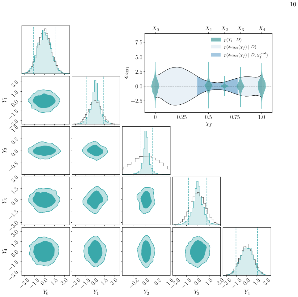
The central claim is that functional deviations from general relativity do not have to be parametrized in advance. The paper shows that a Gaussian process conditioned on a small set of free node values — five nodes on the unit interval with a squared-exponential kernel — combined with the hierarchical likelihood of Eq. (5), reconstructs the relation between $\delta y$ and $\theta_{\mathrm{GR}}$ accurately enough that its 95% credible band is comparable to a parametrized model that contains the true functional relation, at least in regions where the data are informative. The auxiliary variance $\sigma$ in Eq. (4) is what lets the method separate deterministic functional dependence from stochastic departures: its posterior supports $\sigma=0$ for a deterministic underlying relation and shifts away from zero when a stochastic component is injected. Applied to real ringdown measurements of the deviation parameters $\delta\omega_{220}$ and $\delta\omega_{221}$ against the final spin $\chi_f$, the method returns posteriors consistent with no deviation and places upper bounds on $\sigma$.
Load-bearing premise
The load-bearing premise is that the true deviation function varies smoothly, on scales at least as large as the fixed kernel length $l=0.5$, and that the population distribution of the source parameter is Gaussian; if either fails, the reconstructed function will be biased or smoothed out.
Editorial extensions
If this is right
- Agnostic tests can output a map $\delta y(\theta_{\mathrm{GR}})$ instead of a single mean and spread, showing directly where in source-parameter space general relativity might break.
- A $\sigma$ posterior consistent with zero certifies that the deviation relation is deterministic; $\sigma$ away from zero flags environmental or unmodeled stochastic contributions.
- The five-node setup transfers to higher-dimensional parameter spaces and to deviations about an explicit beyond-GR baseline by giving the Gaussian process a nonvanishing mean.
- On real ringdown data the method produces constraints consistent with general relativity and bounds on the stochastic component, so it can serve as a screening tool for systematics in future tests.
Reading between the lines
- The fixed correlation length $l=0.5$ is the main tuning knob: a true deviation varying on scales below this would be smoothed away, so Bayesian model selection over $l$ and kernel choice is a natural next step the authors note but do not implement.
- One could turn the method from a GR-finder into a theory-space explorer by setting a nonvanishing Gaussian-process mean based on a specific beyond-GR waveform family, letting nodes describe fluctuations about that baseline.
- The $\sigma$ parameter may also absorb calibration errors or noise mismodeling in real pipelines, so clean separation of genuine stochastic physics from instrumental systematics will need dedicated validation.
- Because node locations are chosen by the user, the method's output in unsampled regions encodes prior assumptions; comparisons across node placements should accompany any future constraint.
Editorial analysis
A structured set of objections, weighed in public.
Referee Report
Summary. GRANITA is a hierarchical Bayesian method that reconstructs the functional dependence of a gravitational-wave deviation parameter δy on a GR source parameter θGR from individual-event posterior samples. The predictive mean is a Gaussian-process interpolant over a small set of node amplitudes Y_i (Eq. 2), with a squared-exponential kernel whose correlation length is fixed to l=0.5 (Eq. 3), plus an auxiliary variance σ (Eq. 4). The hierarchical likelihood (Eq. 5) reweights each event's posterior by the model prediction and a population distribution p(θGR|β). The method is demonstrated on a toy model with a nonlinear truth (Eq. 1), with and without added stochastic scatter, and applied to public GWTC-3 data: δω220(χf) from 10 pSEOB events and δω221(χf) from 21 pyRing events. Both real-data applications yield null results with σ constrained to small values. The authors claim that in regions with data support, the GRANITA reconstruction is comparable to that of a parametric model containing the true relation.
Significance. The paper addresses a genuine gap: standard agnostic GR tests infer a scalar distribution of deviation parameters but do not reconstruct their functional dependence on source parameters such as mass or spin. The reweighting likelihood (Eq. 5), the use of an auxiliary variance to flag stochastic deviations, and the careful treatment of prior-corrections and MCMC convergence in the real-data application are useful contributions. The toy-model demonstrations are internally consistent, and the comparison with a parametric model that contains the truth is a fair benchmark. The main caveat is that the implemented model is a finite-dimensional smoother with hand-fixed kernel length and node locations; the 'non-perturbative, theory-agnostic' claim is therefore conditional on the chosen smoothing scale rather than being a fully nonparametric procedure. If the authors add robustness checks or hyperparameter inference, the method could be a valuable tool for strong-field tests of GR.
major comments (2)
- [Illustration of the method, Eq. (3) and real-data section] The central demonstration of reconstruction accuracy is made for a truth whose characteristic scale matches the fixed kernel length l=0.5. In Eq. (1), f_true has one sinusoidal oscillation over θ∈[0,1], and the squared-exponential kernel (3) with l=0.5 has a correlation length comparable to the domain. The paper acknowledges in the paragraph after Eq. (3) that l could be optimized by model selection, but the toy demonstration and the GWTC-3 application fix it by hand. A true deviation that varies on a scale shorter than l would be smoothed out and might be absorbed by the auxiliary variance σ, so the claim that GRANITA reconstructs the functional dependence without assuming a functional form is conditional on the smoothing scale. Please add a stress test with a faster-varying truth (e.g., multiple oscillations or a sharp feature) or an evidence-based selection over l and node locations, and report how σ responds in those cases.
- [Supplement, Toy model, and Eq. (2)] The implemented model is not a standard Gaussian process regression with the squared-exponential covariance in Eq. (3). The node values Y_i are assigned independent N(0,1) priors in the supplement, rather than the N(0,K) prior with K_{ij}=k(X_i,X_j) that a GP prior with kernel k would imply. Consequently, μ_pred in Eq. (2) is a linear combination of five fixed basis functions, and the implied prior over functions is a degenerate Gaussian process with covariance k(·,X) K^{-2} k(X,·), not the squared-exponential covariance. The smoothness of the reconstruction is therefore determined entirely by the hand-fixed l and node locations, and the degree of 'non-parametricity' is much more limited than the abstract and introduction suggest. Either use a proper GP prior on the node values (with hyperparameters inferred), or present the method explicitly as a flexible basis-function model and state the limitations of the fixed basis. This is load-bearing for the 'non-perturbative, theory-agnostic' claim.
minor comments (6)
- [Eq. (2)] The notation k^{-1}(X_i,X_j) is confusing; it should be written as (K^{-1})_{ij}, where K_{ij}=k(X_i,X_j), to avoid implying a function k^{-1}.
- [Real-data application, Eq. (5)] The population distribution p(θGR|β)=N(μX,σX) is not truncated to the physical range χf∈[0,1] in the real-data application. Since the final spin is bounded, please justify this choice or use a truncated Gaussian or another bounded distribution.
- [Stochastic toy experiment, Eq. (7)] The statement that the stochastic contribution 'cannot be reduced to a draw from normal distribution' is imprecise: conditional on θ, εQ is normal with variance 0.025^2 θ^4. The actual model mismatch is that the variance depends on θ, whereas the model assumes a constant σ; this is worth stating explicitly.
- [Figure captions and text] There are minor wording issues: 'Further insights is obtained' should be 'Further insight is obtained', and 'posterior model distribution' in the Fig. 1 caption should be 'posterior predictive distribution'.
- [Software and reproducibility] The acknowledgments list Python packages but no code repository; releasing the analysis code would improve reproducibility and is standard for methodological papers in this area.
- [Real-data node selection] The real-data nodes are fixed at {0,0.5,0.65,0.8,1.0}; a sensitivity test with equally spaced nodes or a different l would strengthen the proof-of-concept and address the concern that the results depend on the hand-chosen node layout.
Circularity Check
No significant circularity: GRANITA's reconstruction is validated against injected toy functions and external LVK posteriors, and the only self-citation is a non-load-bearing methodological attribution.
full rationale
The central claim is that GRANITA reconstructs the functional dependence of a deviation parameter on a GR parameter from individual-event posteriors without assuming a functional form. The predictive mean in Eq. (2) is a Gaussian-process interpolation through free node values Y_i, and the posterior over Y_i is obtained from the hierarchical likelihood in Eq. (5) using the individual-event posteriors. The toy-model agreement is checked against f_true from Eq. (1), which was used to generate the mock data; this is standard validation, not circularity. The parametric benchmark in Eq. (6) contains the true model as a special case, but it is used only as a comparison, not as an input to GRANITA. The fixed correlation length l=0.5 (Eq. 3) and hand-placed nodes are explicit modeling assumptions that limit expressivity, but they do not predetermine the inferred functional shape: the node values are data-driven, and the real-data GR-null results are statements about the data under the chosen smoothness scale, not a reduction of the output to the input. The paper's citation of Ref. [33] for the node-parameterization idea is an attribution of technique provenance by a co-author; the derivation here is self-contained in Eqs. (2)-(5), so this self-citation is not load-bearing. No fitted parameter is renamed as a prediction, and no equation reduces to its own inputs by construction. The paper is therefore not circular, though the robustness of the reconstruction to shorter-scale deviations remains an open empirical question.
Assumptions & free parameters
free parameters (5)
- Node values Y_i (toy and real) =
Posterior distributions, not single values
- Auxiliary variance σ =
Posterior bounds, e.g. σ<0.05 at 90% for pSEOB
- Population hyperparameters µX, σX =
Inferred, priors uniform in [0,1]
- Correlation length l =
0.5 fixed
- Node locations Xnodes (real data) =
{0, 0.5, 0.65, 0.8, 1.0}
assumptions (5)
- domain assumption The individual-event priors πi(θGR, δy) are wide and flat so they can be neglected in Eq. (5).
- domain assumption Selection effects are negligible for this analysis.
- domain assumption The population distribution p(θGR|β) is Gaussian with mean and variance in [0,1].
- ad hoc to paper Squared-exponential kernel with fixed correlation length is an adequate prior for the deviation function.
- standard math Standard Gaussian process conditional equations hold (Eq. 2).
Cite this review
Pith. "Pith review of Functional inference on deviations from General Relativity." pith.science (2026). https://pith.science/paper/H4RNBAEX
@misc{pith2026250713454,
  author       = {Pith},
  title        = {Pith review of: Functional inference on deviations from General Relativity},
  year         = {2026},
  howpublished = {\url{https://pith.science/paper/H4RNBAEX}},
  note         = {Machine review of arXiv:2507.13454}
}
read the original abstract
Extensions of general relativity often predict modifications to gravitational waveform morphology that depend functionally on source parameters, such as the masses and spins of coalescing black holes. However, current analyses of strong-field gravity lack robust, data-driven methods to infer such functional dependencies. In this work, we introduce GRANITA, a non-perturbative, theory-agnostic framework to characterize parameter-dependent deviations from general relativity using Gaussian process regression. Leveraging the flexibility of this method, we analyze both simulated data and real events from the LIGO-Virgo-KAGRA public catalog. We demonstrate the ability of our approach to detect and quantify waveform deviations across the parameter space. Furthermore, we show that the method can identify stochastic (non-deterministic) deviations, potentially arising from environmental effects or subdominant unmodeled physics. As gravitational-wave tests of strong gravity advance in precision, our framework provides a principled approach to constrain modified gravity and to mitigate contamination from astrophysical or instrumental systematics.
Figures


Figures from the paper (3 more)


Reference graph
Works this paper leans on
- [1]
- [2]
-
[3]
K. G. Arun, B. R. Iyer, M. S. S. Qusailah, and B. S. Sathyaprakash, Class. Quant. Grav. 23, L37 (2006), arXiv:gr-qc/0604018
arXiv 2006
-
[4]
N. Yunes and F. Pretorius, Phys. Rev. D 80, 122003 (2009), arXiv:0909.3328 [gr-qc]
arXiv 2009
- [5]
- [6]
- [7]
- [8]
Show all 70 references
-
[9]
Ghosh, N
A. Ghosh, N. K. Johnson-Mcdaniel, A. Ghosh, C. K. Mishra, P. Ajith, W. Del Pozzo, C. P. L. Berry, A. B. Nielsen, and L. London, Class. Quant. Grav. 35, 014002 (2018), arXiv:1704.06784 [gr-qc]
2018 arXiv
-
[10]
Bhagwat and C
S. Bhagwat and C. Pacilio, Phys. Rev. D 104, 024030 (2021), arXiv:2101.07817 [gr-qc]
2021 arXiv
-
[11]
Yunes, K
N. Yunes, K. Yagi, and F. Pretorius, Phys. Rev. D 94, 084002 (2016), arXiv:1603.08955 [gr-qc]
2016 arXiv
-
[12]
A. J. K. Chua and M. Vallisneri, (2020), arXiv:2006.08918 [gr-qc]
2020 arXiv
-
[13]
Okounkova, M
M. Okounkova, M. Isi, K. Chatziioannou, and W. M. Farr, Phys. Rev. D 107, 024046 (2023), arXiv:2208.02805 [gr-qc]
2023 arXiv
-
[14]
Juli´ e, L
F.-L. Juli´ e, L. Pompili, and A. Buonanno, Phys. Rev. D 111, 024016 (2025), arXiv:2406.13654 [gr-qc]
2025 arXiv
-
[15]
Pierini and L
L. Pierini and L. Gualtieri, Phys. Rev. D 106, 104009 (2022), arXiv:2207.11267 [gr-qc]
2022 arXiv
-
[16]
H. O. Silva, A. Ghosh, and A. Buonanno, Phys. Rev. D 107, 044030 (2023), arXiv:2205.05132 [gr-qc]
2023 arXiv
-
[17]
Maenaut, G
S. Maenaut, G. Carullo, P. A. Cano, A. Liu, V. Cardoso, T. Hertog, and T. G. F. Li, (2024), arXiv:2411.17893 [gr-qc]
2024 arXiv
-
[18]
Zimmerman, C.-J
A. Zimmerman, C.-J. Haster, and K. Chatziioannou, Phys. Rev. D 99, 124044 (2019), arXiv:1903.11008 [astro-ph.IM]
2019 arXiv
-
[19]
M. Isi, K. Chatziioannou, and W. M. Farr, Phys. Rev. Lett. 123, 121101 (2019), arXiv:1904.08011 [gr-qc]
2019 arXiv
-
[20]
N. K. Johnson-McDaniel, A. Ghosh, S. Ghonge, M. Saleem, N. V. Krishnendu, and J. A. Clark, Phys. Rev. D 105, 044020 (2022), arXiv:2109.06988 [gr-qc]
2022 arXiv
-
[21]
Pacilio, D
C. Pacilio, D. Gerosa, and S. Bhagwat, Phys. Rev. D 109, L081302 (2024), arXiv:2310.03811 [gr-qc]
2024 arXiv
-
[22]
Abbott et al
R. Abbott et al. (LIGO Scientific, Virgo), 103, 122002 (2021), arXiv:2010.14529 [gr-qc]
2021 arXiv
-
[23]
Progetto Dipartimenti di Eccellenza 2023- 2027
to perform GR tests from the pyRing analysis, where δω221 is used as a deviation parameter. Due to higher uncertainties in the posterior contours, we find larger bounds in the 95% confidence region as shown in Fig. 4 (Bottom), as well as on σ (σ <0.18 at 90% credibility), but ...
2021
-
[24]
S. H. V¨ olkel, N. Franchini, and E. Barausse, Phys. Rev. D 105, 084046 (2022), arXiv:2202.08655 [gr-qc]
2022 arXiv
-
[25]
Abbott et al
R. Abbott et al. (LIGO Scientific, VIRGO, KAGRA), (2021), arXiv:2112.06861 [gr-qc]
2021 arXiv
-
[26]
Berti, V
E. Berti, V. Cardoso, and C. M. Will, Phys. Rev. D 73, 064030 (2006), arXiv:gr-qc/0512160
2006 arXiv
-
[27]
Payne, M
E. Payne, M. Isi, K. Chatziioannou, L. Lehner, Y. Chen, and W. M. Farr, Phys. Rev. Lett. 133, 251401 (2024), arXiv:2407.07043 [gr-qc]
2024 arXiv
-
[28]
Maselli, P
A. Maselli, P. Pani, L. Gualtieri, and E. Berti, Phys. Rev. D 101, 024043 (2020), arXiv:1910.12893 [gr-qc]
2020 arXiv
- [29]
-
[30]
Maselli, S
A. Maselli, S. Yi, L. Pierini, V. Vellucci, L. Reali, L. Gualtieri, and E. Berti, Phys. Rev. D 109, 064060 (2024), arXiv:2311.14803 [gr-qc]
2024 arXiv
- [31]
-
[32]
Wang, arXiv e-prints , arXiv:2009.10862 (2020), arXiv:2009.10862 [stat.ML]
J. Wang, arXiv e-prints , arXiv:2009.10862 (2020), arXiv:2009.10862 [stat.ML]
2020 arXiv
-
[33]
C. K. Williams and C. E. Rasmussen, Gaussian processes for machine learning , Vol. 2 (MIT press Cambridge, MA, 2006)
2006
-
[34]
P. S. Cole, G. Bertone, A. Coogan, D. Gaggero, T. Kary- das, B. J. Kavanagh, T. F. M. Spieksma, and G. M. Tomaselli, Nature Astron. 7, 943 (2023), arXiv:2211.01362 [gr-qc]
2023
-
[35]
Pozzoli, R
F. Pozzoli, R. Buscicchio, C. J. Moore, F. Haardt, and A. Sesana, Phys. Rev. D 109, 083029 (2024), arXiv:2311.12111 [astro-ph.CO]
2024 arXiv
-
[36]
Barausse, V
E. Barausse, V. Cardoso, and P. Pani, Phys. Rev. D 89, 104059 (2014), arXiv:1404.7149 [gr-qc]
2014 arXiv
-
[37]
C. A. R. Herdeiro and E. Radu, Int. J. Mod. Phys. D 24, 1542014 (2015), arXiv:1504.08209 [gr-qc]
2015 arXiv
-
[38]
Roy and R
S. Roy and R. Vicente, Phys. Rev. D 111, 084037 (2025), arXiv:2410.16388 [gr-qc]
2025 arXiv
-
[39]
Gupta et al
A. Gupta et al. 10.21468/SciPostPhysCommRep.5 (2024), arXiv:2405.02197 [gr-qc]
2024 arXiv
-
[40]
Payne, M
E. Payne, M. Isi, K. Chatziioannou, and W. M. Farr, Phys. Rev. D 108, 124060 (2023), arXiv:2309.04528 [gr-qc]
2023 arXiv
-
[41]
Caneva Santoro, S
G. Caneva Santoro, S. Roy, R. Vicente, M. Haney, and et al., Phys. Rev. Lett. 132, 251401 (2024), arXiv:2309.05061 [gr-qc]
2024 arXiv
-
[42]
Essick and M
R. Essick and M. Fishbach, Astrophys. J. 962, 169 (2024), arXiv:2310.02017 [gr-qc]
2024 arXiv
-
[43]
We consider a set of 10 GW events that meet the selection criteria detailed in [23]
– a test aiming at performing BH spectroscopy by incorporating pre-merger information. We consider a set of 10 GW events that meet the selection criteria detailed in [23]. We apply granita to characterize a dependence be- tween the deviation parameter δω220 and the final BH sp...
-
[44]
Mandel, W
I. Mandel, W. M. Farr, and J. R. Gair, MNRAS 486, 1086 (2019), arXiv:1809.02063 [physics.data-an]
2019 arXiv
-
[45]
Ghosh, R
A. Ghosh, R. Brito, and A. Buonanno, Phys. Rev. D 103, 124041 (2021), arXiv:2104.01906 [gr-qc]
2021 arXiv
-
[46]
Barausse and T
E. Barausse and T. P. Sotiriou, Class. Quant. Grav. 30, 244010 (2013), arXiv:1307.3359 [gr-qc]
2013 arXiv
-
[47]
Punturo et al., Class
M. Punturo et al., Class. Quant. Grav. 27, 194002 (2010)
2010
-
[48]
Dwyer, D
S. Dwyer, D. Sigg, S. W. Ballmer, L. Barsotti, N. Maval- vala, and M. Evans, Physical Review D 91, 082001 (2015)
2015
-
[49]
B. P. Abbott, R. Abbott, T. D. Abbott, M. R. Abernathy, and et al., Living Reviews in Relativity 21, 3 (2018), arXiv:1304.0670 [gr-qc]
2018 arXiv
-
[50]
Gupta et al
I. Gupta et al. , Class. Quant. Grav. 41, 245001 (2024), arXiv:2307.10421 [gr-qc]
2024 arXiv
- [51]
- [52]
- [53]
-
[54]
Zhong, M
H. Zhong, M. Isi, K. Chatziioannou, and W. M. Farr, Phys. Rev. D 110, 044053 (2024), arXiv:2405.19556 [gr-qc]
2024 arXiv
-
[55]
Saleem, S
M. Saleem, S. Datta, K. G. Arun, and B. S. Sathyaprakash, Phys. Rev. D 105, 084062 (2022), arXiv:2110.10147 [gr- qc]
2022 arXiv
-
[56]
Datta, M
S. Datta, M. Saleem, K. G. Arun, and B. S. Sathyaprakash, Phys. Rev. D 109, 044036 (2024), arXiv:2208.07757 [gr- qc]
2024 arXiv
-
[57]
L. S. Finn and D. F. Chernoff, Phys. Rev. D 47, 2198 (1993), arXiv:gr-qc/9301003 [gr-qc]
1993 arXiv
-
[58]
A. K.-W. Chung and N. Yunes, Phys. Rev. Lett. 133, 181401 (2024), arXiv:2405.12280 [gr-qc]
2024 arXiv
-
[59]
P. A. Cano, L. Capuano, N. Franchini, S. Maenaut, and S. H. V¨ olkel, Phys. Rev. D 110, 124057 (2024), arXiv:2409.04517 [gr-qc]
2024 arXiv
-
[60]
J. L. Bl´ azquez-Salcedo, F. S. Khoo, B. Kleihaus, and J. Kunz, Phys. Rev. D 111, L021505 (2025), arXiv:2407.20760 [gr-qc]
2025 arXiv
-
[61]
Van Rossum and F
G. Van Rossum and F. L. Drake, Python 3 Reference Manual (CreateSpace, 2009)
2009
-
[62]
Foreman-Mackey, The Journal of Open Source Software 1, 24 (2016)
D. Foreman-Mackey, The Journal of Open Source Software 1, 24 (2016)
2016
-
[63]
Frostig, M
R. Frostig, M. J. Johnson, and C. Leary, Systems for Machine Learning 4 (2018)
2018
-
[64]
Bradbury, R
J. Bradbury, R. Frostig, P. Hawkins, M. J. Johnson, C. Leary, D. Maclaurin, G. Necula, A. Paszke, J. Vander- Plas, S. Wanderman-Milne, et al. , Astrophysics Source Code Library , ascl (2021). 7
2021
-
[65]
J. D. Hunter, Computing in Science and Engineering 9, 90 (2007)
2007
-
[66]
D. Phan, N. Pradhan, and M. Jankowiak, arXiv preprint arXiv:1912.11554 (2019)
2019 arXiv
-
[67]
Bingham, J
E. Bingham, J. P. Chen, M. Jankowiak, F. Obermeyer, N. Pradhan, T. Karaletsos, R. Singh, P. A. Szerlip, P. Horsfall, and N. D. Goodman, J. Mach. Learn. Res. 20, 28:1 (2019)
2019
-
[68]
M. D. Hoffman and A. Gelman, arXiv e-prints , arXiv:1111.4246 (2011), arXiv:1111.4246 [stat.CO]
2011 arXiv
-
[69]
Neal, in Handbook of Markov Chain Monte Carlo (2011) pp
R. Neal, in Handbook of Markov Chain Monte Carlo (2011) pp. 113–162
2011
-
[70]
Gelman and D
A. Gelman and D. B. Rubin, Statistical Science 7, 457 (1992). 8 SUPPLEMENT AL MA TERIAL: Analyses details We briefly summarize here some technical details on how we performed the analysis on the toy and GWTC-3 data shown in the main text. To sample the likelihood in Eq. (5) we...
1992
Reviewed August 6, 2026 · model on record in the stance chip above.
Discussion (0). Sign in to comment.