REVIEW 4 major objections 6 minor 60 references
Robustness of analogue Hawking radiation in cavities with moving boundaries
T0 review · 4 major / 6 minor · reviewed 2026-08-06 · deepseek-v4-flash
Pith's one-line read Moving-boundary cavities emit genuine Hawking-like thermal radiation only when one or two symmetrically moving mirrors expand the cavity, and only at low frequencies.
desk verdict Solid negative results, plausible but under-supported positive thermality claims; the core diagnostic is a fit-consistency check, not an independent test. read the letter →
The pith
A machine-rendered reading of the paper's core claim, the machinery that carries it, and where it could break.
The reading
What carries the argument
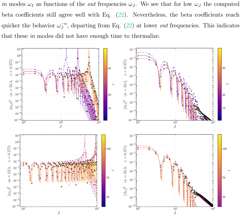
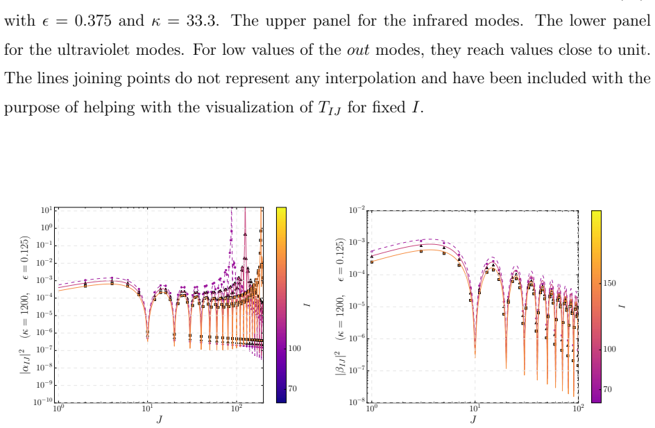
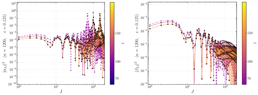
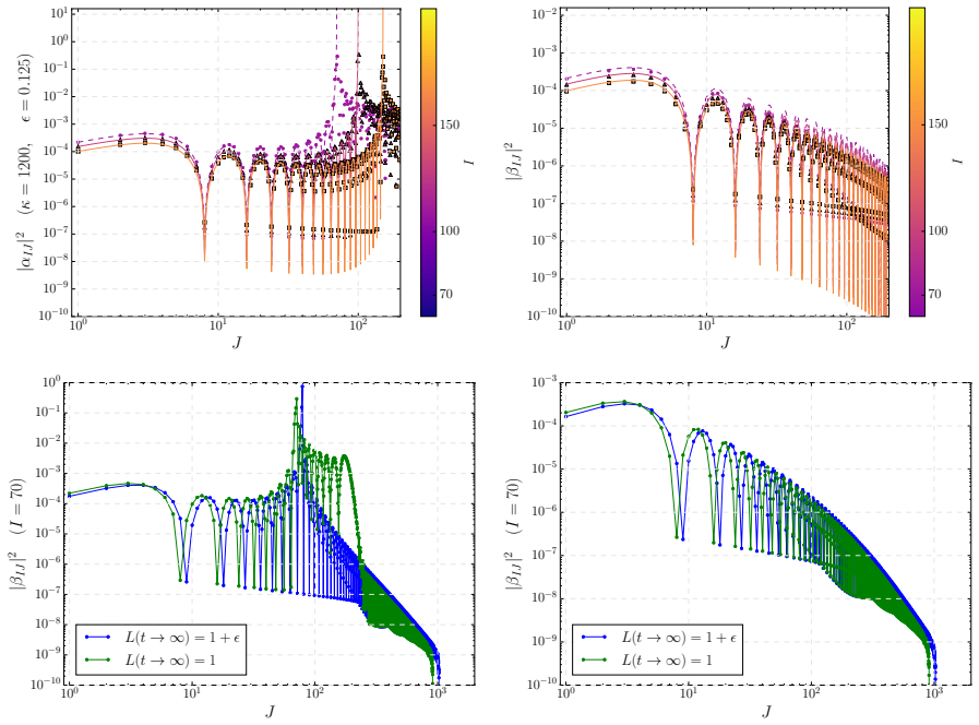
The load-bearing object is the set of Bogoliubov coefficients $\alpha_{IJ}$, $\beta_{IJ}$ connecting the in-vacuum and out-vacuum bases of a massless Klein–Gordon field in a cavity with two moving Dirichlet boundaries. The boundaries couple the Fourier modes through the Hamiltonian in Eq. (5), and the paper integrates the resulting equations with a Prince–Dormand (8,9) Runge–Kutta method, using mode cutoffs $N=256,512,1024$ and Richardson extrapolation toward $N\to\infty$. The thermal claim is carried by two fitting expressions, Eqs. (22) and (24): $|\beta^{(f)}_{IJ}|^2 = N_\beta \Delta\omega_I\Delta\omega_J\, \Gamma_\beta(\epsilon,\omega_J)/(\pi\kappa\omega_I (e^{2\pi\omega_J/\kappa}-1))$ with $\Gamma_\beta(\epsilon,\omega_J)=A_\beta+B_\beta\sin^2(T_\beta\omega_J)$, and an analogous $|\alpha^{(f)}_{IJ}|^2$ containing a resonant factor $1+D_1(F\omega_I)^2/|F\omega_I-\omega_J|^2$. The diagnostic is the thermality function $T_{IJ} = |\alpha_{IJ}|/\bigl[|\beta_{IJ}| e^{\pi\omega_J/\kappa} (1+D_1)^{1/2}(1+D_1(F\omega_I)^2/|F\omega_I-\omega_J|^2)^{1/2}\bigr]$, which equals unity for a mode pair in detailed balance.
What would settle it
Take a deliberately non-thermal boundary trajectory, such as a mirror moving with two incommensurate acceleration pulses, and run the same numerical pipeline with the same fitting expressions. If the fitted gray-body spectrum yields $T_{IJ}\approx1$ in some frequency band, the thermality diagnostic cannot distinguish genuine Hawking-like radiation from a flexible fit; if $T_{IJ}$ remains far from 1, the diagnostic discriminates.
Extended reading notes
Core claim
The paper establishes that thermal particle production in a moving-boundary cavity is real but narrow: in the infrared band, the $|\beta_{IJ}|^2$ coefficients of a one-mirror or two-symmetric-mirror expansion agree with a Fulling–Davies spectrum at temperature $\kappa/2\pi$ once multiplied by the gray-body factor $\Gamma_\beta(\epsilon,\omega_J) = A_\beta + B_\beta \sin^2(T_\beta \omega_J)$, whose sinusoidal oscillations encode the finite duration of the acceleration. The corresponding thermality test $T_{IJ}$, built from the ratio $|\alpha_{IJ}|/|\beta_{IJ}|$ and the fitted resonance denominator $1 + D_1(F\omega_I)^2/|F\omega_I-\omega_J|^2$, reaches values close to unity only for low out-frequencies and low in-modes. By contrast, the time-reversed collapsing trajectories admit no such thermal fit, against the claim of Ref. [58], and a rigidly accelerating cavity fails because its left boundary blue-shifts reflected modes and contaminates the spectrum with ultraviolet quanta. A cavity that returns to its original size after a slow collapse keeps the infrared thermal character, and one or two repeated expansion–collapse cycles preserve the qualitative thermal structure, while beyond three cycles the coefficients grow rapidly and convergence is lost.
Load-bearing premise
The positive thermal claim rests on assuming that a near-unit value of the thermality test, computed with parameters taken from the same gray-body fits whose validity is being tested, indicates a genuine thermal component rather than the flexibility of the fitting formulas, and that the frequency bands selected after seeing the data do not bias the conclusion.
Editorial extensions
If this is right
- Experiments should seek the Hawking-like thermal signal only in expanding cavities with one moving mirror or two symmetrically moving mirrors, and only in infrared modes.
- A collapsing cavity of the type studied here will not emit a thermal spectrum, so a thermal-looking signal from such a configuration would require another explanation.
- Finite-duration acceleration imprints sinusoidal oscillations with period set by $T_\beta=(1+C_\beta)\epsilon$ on the spectrum; these oscillations are a predictable feature, not noise.
- Slowly returning the cavity to its original size preserves the infrared thermal spectrum, and two or three expansion–collapse cycles can be repeated without losing the thermal signature.
- The thermality function $T_{IJ}$ supplies a mode-resolved test that can be applied to experimental Bogoliubov coefficients to separate genuine thermal radiation from boundary artifacts.
Reading between the lines
- A testable extension: because the gray-body period $T_\beta=(1+C_\beta)\epsilon$ should scale linearly with the expansion size at fixed acceleration, measuring the oscillation period for several $\epsilon$ values would test the model independently of the full fit.
- The rigid-cavity failure suggests a design rule the paper leaves implicit: no boundary should be moved in a direction that blue-shifts reflected modes, because those ultraviolet quanta contaminate the infrared thermal signal.
- Whether the instability beyond three cycles is physical parametric amplification or a mode-truncation artifact remains open; an exact analytic trajectory or an adaptive high-cutoff simulation could decide, and the answer determines whether multi-cycle Hawking analogues are feasible at all.
- A direct experimental check of the thermality criterion would compare measured occupation numbers with the fitted coefficients; because Eq. (27) uses parameters from the same fitting expressions under test, an independent measurement is needed to show that $T_{IJ}\approx1$ is not merely self-consistency of the fit.
Editorial analysis
A structured set of objections, weighed in public.
Referee Report
Summary. The manuscript presents a numerical study of a massless scalar field in a 1+1-dimensional cavity with moving Dirichlet boundaries, solving the mode equations with a high-order Runge-Kutta integrator and Richardson extrapolation over mode cutoffs. It surveys expanding, collapsing, rigidly accelerating, and expanding–collapsing trajectories, and proposes fitting expressions (Eqs. (22)–(24)) with gray-body factors to describe deviations from Planckian spectra. The central positive claim is that near-thermal particle production occurs only for low-frequency modes in one-mirror and symmetric two-mirror expanding configurations, with gray-body oscillations set by the acceleration duration; rigid and collapsing configurations are reported as non-thermal, and repeated expansion–collapse cycles are claimed to preserve the thermal structure for a small number of cycles.
Significance. If the claims hold, the paper provides a useful systematic map of parameter regimes in which dynamical Casimir systems can serve as reliable Hawking analogues, with concrete guidance for experiments. The numerical methodology is a genuine strength: the authors use an explicit Dormand–Prince integrator with controlled absolute errors, evolve 256, 512, and 1024 modes, and use Richardson extrapolation to probe the continuum limit. The negative results for rigid and collapsing cavities are supported by raw Bogoliubov coefficients and by the unmodified ratio |alpha_IJ|/(|beta_IJ| e^{pi omega_J/kappa}), so those conclusions are more robust. However, the positive thermality claim rests on fitting diagnostics that are partly circular, so the significance of the paper's main conclusion depends on whether the authors can provide an independent thermality test and quantify fit residuals.
major comments (4)
- [Eq. (27), Sec. III.A] The thermality function T_IJ is not an independent diagnostic. Substituting the fitting forms (22) and (24) on the branch omega_J < F omega_I gives T_IJ^2 = (N_alpha Gamma_alpha)/(N_beta Gamma_beta), because the resonance factor in the alpha-fit is exactly cancelled by the denominator in Eq. (27). In the expanding configurations analyzed in Secs. III.A and III.B the authors set N_alpha = N_beta and Gamma_alpha = Gamma_beta (e.g., A_alpha = A_beta = 1, B_alpha = B_beta = 10^{-3}, C_alpha = C_beta), so T_IJ = 1 identically for any numerical data that match the fitted functional form, independently of whether the state is actually thermal. Figures 2, 4, 6, and 8 therefore primarily demonstrate fit self-consistency and selected frequency bands, not an independent verification of detailed balance. Please report the unmodified ratio |alpha_IJ|/(|beta_IJ| e^{pi omega_J/kappa}) together with residuals, and state the criterion used to select the modes shown.
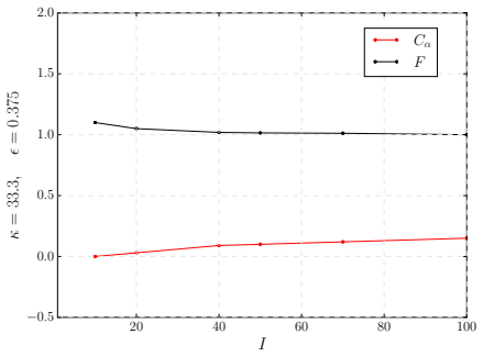
- [Eqs. (22)–(24), Appendix A] The central positive claim is supported by fitting expressions with a large number of free parameters—N_alpha, N_beta, A, B, C, D1, D2, F, and kappa_tilde—but no residuals, confidence intervals, or goodness-of-fit statistics are reported. The same functional forms are both the object of the thermality test and the source of the correction factors in Eq. (27). Because the fits can absorb non-Planckian structure, the statement that deviations are 'quantified' requires an error analysis. Please provide residuals as a function of (I,J) for the displayed bands and justify the ansatz Gamma = A + B sin^2(T omega_J) against alternative functional forms.
- [Sec. III, paragraph after Eq. (23)] The parametrization is applied only to 'the sets of modes that reach a nearly thermal final state,' and modes in which |beta_IJ| departs from the fit are explicitly excluded ('we do not consider them here') in Secs. III.A and III.B. This post-hoc band selection can bias the conclusion toward thermality. Please quantify how many modes are excluded, show the full I x J region, and test whether the conclusions change when the selection criterion is varied.
- [Secs. V.A–V.C] The robustness claim for expansion–collapse cycles is not supported by the same standard as the single-expansion claim. In Sec. V.A the fitting expressions are said to apply 'only for infrared modes,' and in Sec. V.C Richardson convergence is lost already at the third cycle ('we lost convergence in the infrared sector... amplitudes grow very rapidly'). The statement that the thermal structure persists for fewer than three cycles is not accompanied by a T_IJ or residual analysis for the composed Bogoliubov coefficients. Please provide a quantitative thermality diagnostic for the composed transformations or soften the claim accordingly.
minor comments (6)
- [Abstract] 'Dinamical Casimir effect' should be 'Dynamical Casimir effect'.
- [Fig. 12 caption] The caption refers to Eq. (28), but the rigid-cavity trajectory analyzed in that section is given by Eq. (29).
- [Sec. III.A, large accelerations] The sentence 'the computed beta coefficients agree very well with Eqs. (24) and (22)' appears to ascribe the beta coefficients to Eq. (24); the intended statement is likely that alpha coefficients match Eq. (24) and beta coefficients match Eq. (22).
- [Fig. 21 caption] 'D!' should read 'D1'.
- [Sec. III.A, after Eq. (27)] The text 'we show the thermal relation TIJ in Eq. (2)' should refer to Eq. (27), not Eq. (2).
- [Sec. II] 'Poison algebra' should be 'Poisson algebra'.
Circularity Check
The thermality diagnostic T_IJ in Eq. (27) cancels by construction the fitted correction of the alpha spectrum, so T_IJ ~ 1 partly reflects self-consistency of the fits in Eqs. (22)-(24) plus post-hoc selection of 'nearly thermal' bands.
-
fitted input called prediction
[Section III.A and III.B, Eqs. (22), (24), and (27)]
"Instead, our point of view is that one should check whether the following thermality function TIJ = |αIJ|/(|βIJ| e^{πωJ/κ}) (1+D1)^{1/2}/(1 + D1 (FωI)^2/|FωI−ωJ|^2)^{1/2}, equals unit. It will agree with the standard one in the limit F ωI ≫ ωJ anyways."
D1 and F in Eq. (27) are fitted parameters from the alpha fitting expression (24). If the numerical data obey both fits (22) and (24) on the branch ωJ < FωI, substitution gives T_IJ^2 = (N_alpha Gamma_alpha)/(N_beta Gamma_beta). In the expanding configurations the paper sets N_alpha = N_beta and Gamma_alpha = Gamma_beta (e.g., A_alpha = A_beta = 1, B_alpha = B_beta = 10^-3, C_alpha = C_beta), so T_IJ = 1 identically. The diagnostic therefore measures consistency with the paper's own fitted template, not an independent detailed-balance test; near-unity T_IJ for modes already used to fix the fits is not independent evidence of thermality.
-
self definitional
[Section III, paragraph following Eqs. (22)-(24); Section III.B large accelerations]
"This parametrization is valid only for the sets of modes that reach a nearly thermal final state. These sets of thermal modes will depend on the trajectories of the mirrors. An exact thermal state will correspond to Γβ(ϵ, ωJ) = 1."
The domain of validity of the fitting parametrization is defined as 'modes that reach a nearly thermal final state' — the very property the fits are used to establish. Modes whose beta coefficients depart from the thermal template are then explicitly excluded ('those modes depart strongly from a thermal distribution, and hence we do not consider them here'). Thus the reported agreement between data, fits, and T_IJ near one is, for the retained bands, enforced by the selection criterion rather than discovered independently.
full rationale
The paper contains substantial independent numerical content: the Bogoliubov coefficients are obtained by solving the coupled ODEs (8)-(9) with high-precision methods, and the negative thermality conclusions for rigid and collapsing cavities do not rely on the questioned diagnostic in the same way. However, the central positive claim ('thermal signatures emerge in specific expanding cavity configurations') is validated through the thermality function T_IJ of Eq. (27), which is normalized by the fitted parameters D1 and F of Eq. (24). Under the paper's own fitting forms, T_IJ reduces to sqrt(N_alpha Gamma_alpha/(N_beta Gamma_beta)), and in all expanding configurations reported as thermal the authors fix the norms and gray-body parameters equal for alpha and beta, so T_IJ is 1 whenever the data match the fits — regardless of whether the state is thermal. The independent Davies-Fulling detailed-balance test (3) is replaced by this self-normalized version. A second, narrower circularity is the post-hoc restriction of the parametrization to modes that already 'reach a nearly thermal final state'. Weighing these issues, the positive thermality claim is partially circular (score 6), but the negative results and the raw numerical spectra retain independent value. Self-citations such as Ref. [48] are used as motivation rather than as load-bearing proof, so they do not add to the score.
Assumptions & free parameters
free parameters (11)
- A_beta (gray-body offset for beta) =
1.0 (set to 1 in most simulations)
- B_beta (gray-body oscillation amplitude for beta) =
10^-3 (small accel), 10^-4 to 10^-3 (large accel)
- C_beta (gray-body period parameter for beta) =
~0 for small accelerations, ~1.0 for large accelerations
- A_alpha (gray-body offset for alpha) =
1.0
- B_alpha (gray-body oscillation amplitude for alpha) =
10^-3
- C_alpha (gray-body period parameter for alpha) =
~0 to 1.0
- D1 (resonance denominator parameter) =
0.1
- D2 (resonance denominator parameter, high-frequency branch) =
0.1
- F (frequency shift parameter) =
O(1), plotted vs omega_I
- kappa_tilde (modified acceleration or temperature) =
1.6 kappa (small accel case)
- N_alpha, N_beta (normalization factors) =
2 (one mirror), 4 (symmetric two mirrors)
assumptions (5)
- standard math Klein-Gordon mode decomposition and Bogoliubov transformation formalism for a massless scalar field in a 1+1 cavity with moving Dirichlet boundaries
- domain assumption Cavity is static in the asymptotic past and future, so in and out vacua are well-defined
- domain assumption Davies-Fulling detailed balance condition |alpha|^2 = e^{2 pi omega / kappa} |beta|^2 is a valid signature of thermal equilibrium at T = kappa / (2 pi)
- domain assumption Richardson extrapolation from mode cutoffs N = 256, 512, 1024 converges to the N to infinity result in the frequency bands used for thermality
- ad hoc to paper Gray-body factor Gamma(epsilon, omega_J) = A + B sin^2(T omega_J) is the correct functional form for finite-size and transient deviations
Cite this review
Pith. "Pith review of Robustness of analogue Hawking radiation in cavities with moving boundaries." pith.science (2026). https://pith.science/paper/23NHCM6M
@misc{pith2026250713894,
  author       = {Pith},
  title        = {Pith review of: Robustness of analogue Hawking radiation in cavities with moving boundaries},
  year         = {2026},
  howpublished = {\url{https://pith.science/paper/23NHCM6M}},
  note         = {Machine review of arXiv:2507.13894}
}
read the original abstract
In this work we explore the limitations and robustness of thermal radiation in dynamical Casimir systems serving as analogs for Hawking radiation. Through detailed numerical analysis, we characterize particle production spectra in cavities with moving boundaries under various configurations, including expanding, collapsing, and rigidly accelerating scenarios. We find that thermal signatures emerge in specific expanding cavity configurations but are highly dependent on frequency bands and acceleration parameters. In those configurations of the cavity where there is thermal production, we derive fitting expressions that quantify deviations from idealized thermal spectra through gray-body factors, revealing oscillatory behaviors tied to acceleration duration. Our results identify which experimental setups can reliably simulate gravitationally-induced phenomena and quantify how finite-size effects and transient dynamics modify the expected thermal distributions, providing a comprehensive framework for distinguishing genuine Hawking-like radiation from experimental artifacts.
Figures


Figures from the paper (20 more)









Reference graph
Works this paper leans on
-
[1]
S. W. Hawking, Communications in Mathematical Physics 43, 199 (1975)
work page 1975
-
[2]
W. G. Unruh, Physical Review D 14, 870 (1976)
work page 1976
-
[3]
P. C. W. Davies and S. A. Fulling, Proceedings of the Royal Society of London. A. Mathe- matical and Physical Sciences 356, 237 (1977)
work page 1977
-
[4]
N. D. Birrell and P. C. W. Davies, Quantum fields in curved space (Cambridge University Press, 1982)
work page 1982
-
[5]
L. J. Garay, J. R. Anglin, J. I. Cirac, and P. Zoller, Phys. Rev. Lett. 85, 4643 (2000), arXiv:gr-qc/0002015
arXiv 2000
- [6]
-
[7]
C. Barcelo, S. Liberati, and M. Visser, Int. J. Mod. Phys. A 18, 3735 (2003), arXiv:gr- qc/0110036
-
[8]
J. Steinhauer, Nature Phys. 12, 959 (2016), arXiv:1510.00621 [gr-qc]
arXiv 2016
Show all 60 references
-
[9]
Mu˜ noz de Nova, K
J. Mu˜ noz de Nova, K. Golubkov, V. Kolobov, and et al., Nature 569, 688 (2019), arXiv:1809.00913
2019 arXiv
-
[10]
V. I. Kolobov, K. Golubkov, J. R. Mu˜ noz de Nova, and J. Steinhauer, Nature Phys. 17, 362 (2021), arXiv:1910.09363 [gr-qc]
2021
-
[11]
Leonhardt, Annalen Phys
U. Leonhardt, Annalen Phys. 530, 1700114 (2018), arXiv:1609.03803 [gr-qc]
2018 arXiv
-
[12]
Steinhauer, Annalen Phys
J. Steinhauer, Annalen Phys. 530, 1700459 (2018)
2018
-
[13]
Schutzhold and W
R. Schutzhold and W. G. Unruh, Phys. Rev. D 66, 044019 (2002), arXiv:gr-qc/0205099
2002 arXiv
-
[14]
Rousseaux, C
G. Rousseaux, C. Mathis, P. Maissa, T. G. Philbin, and U. Leonhardt, New J. Phys. 10, 053015 (2008), arXiv:0711.4767 [gr-qc]
2008 arXiv
-
[15]
Weinfurtner, E
S. Weinfurtner, E. W. Tedford, M. C. J. Penrice, W. G. Unruh, and G. A. Lawrence, Phys. Rev. Lett. 106, 021302 (2011), arXiv:1008.1911 [gr-qc]
2011 arXiv
-
[16]
Weinfurtner, E
S. Weinfurtner, E. W. Tedford, M. C. J. Penrice, W. G. Unruh, and G. A. Lawrence, Lect. Notes Phys. 870, 167 (2013), arXiv:1302.0375 [gr-qc]
2013 arXiv
-
[17]
Michel and R
F. Michel and R. Parentani, Phys. Rev. D 90, 044033 (2014), arXiv:1404.7482 [gr-qc]
2014 arXiv
-
[18]
Coutant and S
A. Coutant and S. Weinfurtner, Phys. Rev. D 94, 064026 (2016), arXiv:1603.02746 [gr-qc]
2016 arXiv
-
[19]
Euv´ e, F
L.-P. Euv´ e, F. Michel, R. Parentani, and G. Rousseaux, Phys. Rev. D 91, 024020 (2015), arXiv:1409.3830 [gr-qc]
2015 arXiv
-
[20]
L. P. Euv´ e, F. Michel, R. Parentani, T. G. Philbin, and G. Rousseaux, Phys. Rev. Lett. 117, 121301 (2016), arXiv:1511.08145 [physics.flu-dyn]
2016 arXiv
-
[21]
Euv´ e, S
L.-P. Euv´ e, S. Robertson, N. James, A. Fabbri, and G. Rousseaux, Phys. Rev. Lett. 124, 141101 (2020), arXiv:1806.05539 [gr-qc]
2020 arXiv
-
[22]
Schutzhold and W
R. Schutzhold and W. G. Unruh, Phys. Rev. Lett. 95, 031301 (2005), arXiv:quant-ph/0408145
2005 arXiv
-
[23]
T. G. Philbin, C. Kuklewicz, S. Robertson, S. Hill, F. Konig, and U. Leonhardt, Science 319, 1367 (2008), arXiv:0711.4796 [gr-qc]
2008 arXiv
-
[24]
Belgiorno, S
F. Belgiorno, S. L. Cacciatori, G. Ortenzi, V. G. Sala, and D. Faccio, Phys. Rev. Lett. 104, 140403 (2010)
2010
-
[25]
Rubino, F
E. Rubino, F. Belgiorno, S. L. Cacciatori, M. Clerici, V. Gorini, G. Ortenzi, L. Rizzi, V. G. 38 Sala, M. Kolesik, and D. Faccio, New J. Phys. 13, 085005 (2011)
2011
-
[26]
Drori, Y
J. Drori, Y. Rosenberg, D. Bermudez, Y. Silberberg, and U. Leonhardt, Phys. Rev. Lett. 122, 010404 (2019), arXiv:1808.09244 [gr-qc]
2019 arXiv
-
[27]
Carusotto and C
I. Carusotto and C. Ciuti, Phys. Rev. Lett. 93, 166401 (2004)
2004
-
[28]
H. S. Nguyen, D. Gerace, I. Carusotto, D. Sanvitto, E. Galopin, A. Lema ˆ ıtre, I. Sagnes, J. Bloch, and A. Amo, Phys. Rev. Lett. 114, 036402 (2015)
2015
-
[29]
Falque, A
K. Falque, A. Delhom, Q. Glorieux, E. Giacobino, A. Bramati, and M. J. Jacquet, Phys. Rev. Lett. 135, 023401 (2025), arXiv:2311.01392 [cond-mat.quant-gas]
2025 arXiv
-
[30]
G. T. Moore, Journal of Mathematical Physics 11, 2679 (1970)
1970
-
[31]
V. V. Dodonov, MDPI Physics 7, 10 (2025)
2025
-
[32]
R. D. Carlitz and R. S. Willey, Physical Review D 36, 2327 (1987)
1987
-
[33]
Friis, D
N. Friis, D. E. Bruschi, J. Louko, and I. Fuentes, Phys. Rev. D 85, 081701 (2012), arXiv:1201.0549 [quant-ph]
2012 arXiv
-
[34]
P. M. Alsing and I. Fuentes, Classical and Quantum Gravity 29, 224001 (2012)
2012
-
[35]
D. E. Bruschi, J. Louko, D. Faccio, and I. Fuentes, New J. Phys. 15, 073052 (2013), arXiv:1210.6772 [quant-ph]
2013 arXiv
-
[36]
Lindkvist, C
J. Lindkvist, C. Sab ´ ın, I. Fuentes, A. Dragan, I.-M. Svensson, P. Delsing, and G. Johansson, Phys. Rev. A 90, 052113 (2014), arXiv:1401.0129 [quant-ph]
2014 arXiv
-
[37]
Sab ´ ın and G
C. Sab ´ ın and G. Adesso, Phys. Rev. A92, 042107 (2015), arXiv:1506.09001 [quant-ph]
2015 arXiv
-
[38]
Romualdo, L
I. Romualdo, L. Hackl, and N. Yokomizo, Phys. Rev. D 100, 065022 (2019), arXiv:1908.00835 [quant-ph]
2019 arXiv
-
[39]
N. F. Del Grosso, F. C. Lombardo, and P. I. Villar, Phys. Rev. D 102, 125008 (2020), arXiv:2007.06627 [quant-ph]
2020 arXiv
-
[40]
W. Cong, E. Tjoa, and R. B. Mann, JHEP 06, 021 (2019), [Erratum: JHEP 07, 051 (2019)], arXiv:1810.07359 [quant-ph]
2019 arXiv
-
[41]
T. R. Perche, J. Polo-G´ omez, B. de S. L. Torres, and E. Mart ´ ın-Mart ´ ınez, Phys. Rev. D109, 045018 (2024), arXiv:2310.18432 [quant-ph]
2024 arXiv
-
[42]
Ragula, B
B. Ragula, B. de S. L. Torres, E. Schnetter, and E. Mart ´ ın-Mart ´ ınez, Phys. Rev. D 111, 105029 (2025), arXiv:2502.02643 [quant-ph]
2025 arXiv
-
[43]
Chen, H.-F
W. Chen, H.-F. Li, Z.-Y. Wu, L.-Y. Gong, X. Wu, P.-M. Jiang, X.-G. Zheng, and D.-Z. Yao, Scientific Reports 7, 17011 (2017). 39
2017
-
[44]
C. M. Wilson, G. Johansson, A. Pourkabirian, M. Simoen, J. R. Johansson, T. Duty, F. Nori, and P. Delsing, Nature 479, 376 (2011)
2011
-
[45]
Terrones and C
A. Terrones and C. Sab ´ ın, Universe7, 499 (2021), arXiv:2110.11344 [gr-qc]
2021 arXiv
-
[46]
M. D. Maceda and C. Sab ´ ın, Sci. Rep.15, 20626 (2025)
2025
-
[47]
Garc ´ ıa Mart ´ ın-Caro, G
A. Garc ´ ıa Mart ´ ın-Caro, G. Garc ´ ıa-Moreno, J. Olmedo, and J. M. S´ anchez Vel´ azquez, Phys. Rev. D 110, 025007 (2024), arXiv:2404.06166 [quant-ph]
2024 arXiv
-
[48]
Garc ´ ıa Mart ´ ın-Caro, G
A. Garc ´ ıa Mart ´ ın-Caro, G. Garc ´ ıa-Moreno, J. Olmedo, and J. M. S´ anchez Vel´ azquez, Phys. Rev. D 108, L061701 (2023), arXiv:2306.05250 [gr-qc]
2023 arXiv
-
[49]
M. R. R. Good, P. R. Anderson, and C. R. Evans, Phys. Rev. D 88, 025023 (2013), arXiv:1303.6756 [gr-qc]
2013 arXiv
-
[50]
L¨ ahteenm¨ aki, G
P. L¨ ahteenm¨ aki, G. S. Paraoanu, J. Hassel, and P. J. Hakonen, Proceedings of the National Academy of Sciences 110, 4234 (2013)
2013
-
[51]
P. D. Nation, J. R. Johansson, M. P. Blencowe, and F. Nori, Reviews of Modern Physics 84, 1 (2012)
2012
-
[52]
Haro, Journal of Physics A: Mathematical and General 38, L307 (2005)
J. Haro, Journal of Physics A: Mathematical and General 38, L307 (2005)
2005
-
[53]
Haro and E
J. Haro and E. Elizalde, J. Phys. A 41, 032002 (2008), arXiv:0709.3638 [quant-ph]
2008 arXiv
-
[54]
R. Kubo, J. Phys. Soc. Jap. 12, 570 (1957)
1957
-
[55]
P. C. Martin and J. Schwinger, Phys. Rev. 115, 1342 (1959)
1959
-
[56]
Takagi, Prog
S. Takagi, Prog. Theor. Phys. Suppl. 88, 1 (1986)
1986
-
[57]
Carballo-Rubio, L
R. Carballo-Rubio, L. J. Garay, E. Mart ´ ın-Mart ´ ınez, and J. de Ram´ on, Phys. Rev. Lett.123, 041601 (2019)
2019
-
[58]
Castagnino and R
M. Castagnino and R. Ferraro, Annals of Physics 154, 1 (1984)
1984
-
[59]
Mujtaba, E
A. Mujtaba, E. Ievlev, M. J. Gorban, and M. R. R. Good, Phys. Rev. D 111, 065011 (2025), arXiv:2411.03521 [quant-ph]. 40
2025 arXiv
-
[1200]
Other configurations with large accelerations show similar results. In Fig. 3 we show the behavior of the Bogoliubov coefficients for modes in the frequency bandI ∈ (70, 150) and J ∈ (1, 150), and compare them with the fitting expression of Eq.(22). In these simulations, we se...
Reviewed August 6, 2026 · model on record in the stance chip above.
Discussion (0). Sign in to comment.