Frabjous: Deep Learning Fast Radio Burst Morphologies
Pith reviewed 2026-05-19 04:35 UTC · model grok-4.3
The pith
Deep learning trained on simulated and real data classifies fast radio burst morphologies at 55 percent accuracy.
A machine-rendered reading of the paper's core claim, the machinery that carries it, and where it could break.
Core claim
Frabjous applies deep learning to FRB morphology classification by combining simulated examples with real observations from the CHIME/FRB catalog, resulting in an overall classification accuracy of approximately 55 percent for five balanced classes during training.
What carries the argument
The Frabjous deep learning model trained on a hybrid dataset of simulated FRB signals and real catalog entries.
If this is right
- Automated morphology classification can help prioritize limited multi-wavelength follow-up resources for the most interesting FRBs.
- Statistical analysis of FRB morphologies becomes feasible with growing detection rates.
- Performance can be improved by augmenting training datasets and refining simulation strategies.
Where Pith is reading between the lines
- Similar simulation-augmented training could benefit classification tasks in other areas with sparse labeled astronomical data.
- Extending the model to handle more classes or continuous morphology parameters might reveal new patterns in FRB populations.
- Integration with real-time detection pipelines could enable immediate anomaly flagging as new surveys increase event rates.
Load-bearing premise
The simulations used to generate additional training examples accurately capture the diversity and characteristics of real FRB morphologies observed in the CHIME/FRB catalog.
What would settle it
Evaluating the trained model on a held-out set of newly observed real FRBs with independently determined morphologies and checking whether the accuracy remains above 50 percent.
Figures


read the original abstract
The increasing field of view of radio telescopes and improved data processing capabilities have led to a surge in the detection of Fast Radio Bursts (FRBs). The discovery rate of FRBs is already a few per day and is expected to increase rapidly with new surveys coming online. The growing number of events necessitates prioritized follow-up due to limited multi-wavelength resources, requiring rapid and automated classification. In this study, we introduce Frabjous, a deep learning framework for an automated morphology classifier with an aim towards enabling the prompt follow-up of anomalous and intriguing FRBs, and a comprehensive statistical analysis of FRB morphologies. Deep learning models require a large training set of each FRB archetype, however, publicly available data lacks sufficient samples for most FRB types. In this paper, we build a simulation framework for generating realistic examples of FRBs and train a network based on a combination of simulated and real data, starting with the CHIME/FRB catalog. Applying our framework to the first CHIME/FRB catalog, we achieve an overall classification accuracy of approximately 55%, well over a random multiclass classification rate of 20 % with five balanced classes during training. While this falls short of desirable performance, we critically discuss the limitations of our approach and propose potential avenues for improvement. Future work should explore strategies to augment training datasets and broaden the scope of FRB morphological studies, aiming for more accurate and reliable classification results.
Editorial analysis
A structured set of objections, weighed in public.
Referee Report
Summary. The manuscript introduces Frabjous, a deep learning framework for automated classification of Fast Radio Burst (FRB) morphologies. To overcome limited labeled real data, the authors develop a simulation framework to generate additional training examples and combine these with real events from the first CHIME/FRB catalog. They train a network on the augmented dataset for five morphology classes and report an overall classification accuracy of approximately 55%, exceeding the 20% random baseline. The authors explicitly note that performance falls short of desirable levels, discuss limitations, and outline potential improvements for dataset augmentation and broader morphological studies.
Significance. If the simulations are shown to reproduce the statistical properties of real FRB morphologies, the framework could provide a practical route to automated classification tools that help prioritize limited multi-wavelength follow-up resources as detection rates rise. The strategy of augmenting scarce real data with targeted simulations directly addresses a common bottleneck in radio transient studies and supplies a concrete baseline (55% vs. 20%) against which future refinements can be measured.
major comments (1)
- [Simulation framework and training procedure] The central claim of ~55% accuracy on the CHIME/FRB catalog (abstract) requires that simulated training examples capture the morphological statistics (width, scattering, spectral structure, noise) of real events sufficiently well for the network to learn transferable features. No quantitative validation metrics—such as parameter-distribution overlap, expert visual scoring, or domain-adversarial distances—are reported for the five classes. Without these checks, the improvement over the random baseline could reflect simulation-specific artifacts rather than genuine generalization to the catalog.
minor comments (1)
- [Abstract] The abstract states that five balanced classes were used during training but does not name the morphological archetypes; adding the class labels would aid readers who are not already familiar with the FRB morphology taxonomy.
Simulated Author's Rebuttal
We thank the referee for their constructive and insightful comments on our manuscript. We have carefully considered the major comment and provide a detailed response below. We believe the suggested revisions will improve the rigor of our presentation of the simulation framework.
read point-by-point responses
-
Referee: The central claim of ~55% accuracy on the CHIME/FRB catalog (abstract) requires that simulated training examples capture the morphological statistics (width, scattering, spectral structure, noise) of real events sufficiently well for the network to learn transferable features. No quantitative validation metrics—such as parameter-distribution overlap, expert visual scoring, or domain-adversarial distances—are reported for the five classes. Without these checks, the improvement over the random baseline could reflect simulation-specific artifacts rather than genuine generalization to the catalog.
Authors: We agree that quantitative validation of the simulated morphologies against real events is essential to substantiate the transferability of learned features and to rule out simulation-specific artifacts. The current manuscript discusses limitations of the approach and notes that the 55% accuracy falls short of desirable performance, but does not include the specific metrics suggested. In the revised manuscript we will add direct comparisons of key parameter distributions (burst width, scattering timescale, spectral index, and noise properties) between simulated and real FRBs for each of the five morphology classes, including summary statistics and overlap measures such as Kolmogorov-Smirnov tests. We will also include a small-scale expert visual scoring exercise on a representative subset of simulated events. While full implementation of domain-adversarial distance metrics would require substantial additional computational work, we will expand the limitations and future-work sections to discuss this technique as a promising direction for further validation. These additions will be incorporated in the next version of the paper. revision: yes
Circularity Check
No circularity: empirical ML accuracy on external catalog data
full rationale
The paper describes a standard supervised deep learning pipeline: a simulation framework generates additional training examples of FRB morphologies, which are combined with real CHIME/FRB catalog events to train a classifier. The reported ~55% accuracy is an empirical evaluation metric on the catalog, not the output of any equation or parameter fit that reduces to the training inputs by construction. No self-definitional steps, fitted inputs renamed as predictions, load-bearing self-citations, or ansatzes appear in the derivation chain. The result depends on data and model training rather than tautological re-expression of its own assumptions.
Axiom & Free-Parameter Ledger
free parameters (2)
- Number of morphological classes
- Simulation hyperparameters
axioms (1)
- domain assumption Simulated FRB signals can be made sufficiently realistic to augment limited real data for training a morphology classifier.
Lean theorems connected to this paper
-
IndisputableMonolith/Cost/FunctionalEquation.leanwashburn_uniqueness_aczel unclear?
unclearRelation between the paper passage and the cited Recognition theorem.
We build a simulation framework for generating realistic examples of FRBs and train a network based on a combination of simulated and real data... overall classification accuracy of approximately 55%
-
IndisputableMonolith/Foundation/RealityFromDistinction.leanreality_from_one_distinction unclear?
unclearRelation between the paper passage and the cited Recognition theorem.
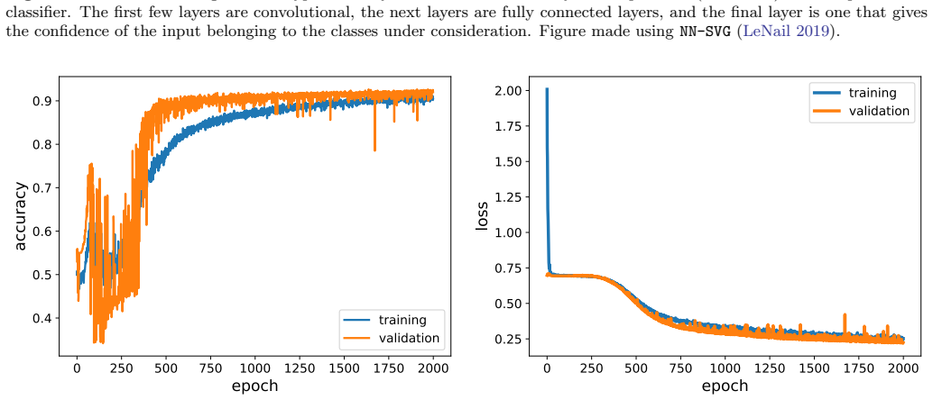
We use keras and tensorflow... first few layers are CNN layers to extract local features
What do these tags mean?
- matches
- The paper's claim is directly supported by a theorem in the formal canon.
- supports
- The theorem supports part of the paper's argument, but the paper may add assumptions or extra steps.
- extends
- The paper goes beyond the formal theorem; the theorem is a base layer rather than the whole result.
- uses
- The paper appears to rely on the theorem as machinery.
- contradicts
- The paper's claim conflicts with a theorem or certificate in the canon.
- unclear
- Pith found a possible connection, but the passage is too broad, indirect, or ambiguous to say the theorem truly supports the claim.
Reference graph
Works this paper leans on
-
[1]
2015, TensorFlow: Large-Scale Machine Learning on Heterogeneous Systems
Abadi, M., Agarwal, A., Barham, P., et al. 2015, TensorFlow: Large-Scale Machine Learning on Heterogeneous Systems. https://www.tensorflow.org/
work page 2015
-
[2]
2016, in 12th {USENIX} Symposium on Operating Systems Design and Implementation ({OSDI} 16), 265–283
Abadi, M., Barham, P., Chen, J., et al. 2016, in 12th {USENIX} Symposium on Operating Systems Design and Implementation ({OSDI} 16), 265–283
work page 2016
-
[3]
C., Buffaz, E., Vieira, N., et al
Abbott, T. C., Buffaz, E., Vieira, N., et al. 2022, ApJ, 927, 232, doi: 10.3847/1538-4357/ac5019
-
[4]
Agarwal, D., & Aggarwal, K. 2020, FETCH: Fast Extragalactic Transient Candidate Hunter, Astrophysics Source Code Library, record ascl:2005.014. http://ascl.net/2005.014
work page 2020
-
[5]
Agarwal, D., Aggarwal, K., Burke-Spolaor, S., Lorimer, D. R., & Garver-Daniels, N. 2020, MNRAS, 497, 1661, doi: 10.1093/mnras/staa1856
-
[6]
2020, ApJ, 888, 40, doi: 10.3847/1538-4357/ab5363
Balasubramanian, A. 2020, ApJ, 888, 40, doi: 10.3847/1538-4357/ab5363
-
[7]
BEiT: BERT Pre-Training of Image Transformers
Bao, H., Dong, L., Piao, S., & Wei, F. 2021, arXiv e-prints, arXiv:2106.08254, doi: 10.48550/arXiv.2106.08254
work page internal anchor Pith review Pith/arXiv arXiv doi:10.48550/arxiv.2106.08254 2021
-
[8]
Bassa, C. G., Tendulkar, S. P., Adams, E. A. K., et al. 2017, ApJL, 843, L8, doi: 10.3847/2041-8213/aa7a0c
-
[9]
Bhandari, S., Sadler, E. M., Prochaska, J. X., et al. 2020, ApJL, 895, L37, doi: 10.3847/2041-8213/ab672e
-
[10]
Bochenek, C. D., Ravi, V., Belov, K. V., et al. 2020, Nature, 587, 59, doi: 10.1038/s41586-020-2872-x
-
[11]
2022, Nature Astronomy, 6, 828, doi: 10.1038/s41550-022-01688-x
Caleb, M., Heywood, I., Rajwade, K., et al. 2022, Nature Astronomy, 6, 828, doi: 10.1038/s41550-022-01688-x
-
[12]
2023, arXiv e-prints, arXiv:2307.09502, doi: 10.48550/arXiv.2307.09502
Cassanelli, T., Leung, C., Sanghavi, P., et al. 2023, arXiv e-prints, arXiv:2307.09502, doi: 10.48550/arXiv.2307.09502
-
[13]
2017, Nature, 541, 58, 10.1038/nature20797
Chatterjee, S., Law, C. J., Wharton, R. S., et al. 2017, Nature, 541, 58, doi: 10.1038/nature20797
-
[14]
H., Hashimoto, T., Goto, T., et al
Chen, B. H., Hashimoto, T., Goto, T., et al. 2022, MNRAS, 509, 1227, doi: 10.1093/mnras/stab2994 —. 2023, MNRAS, 521, 5738, doi: 10.1093/mnras/stad930
-
[15]
Chen, S., Shu, T., Zhao, H., & Tang, Y. Y. 2023, Knowledge-Based Systems, 278, 110881, doi: https://doi.org/10.1016/j.knosys.2023.110881 CHIME/FRB Collaboration, Amiri, M., Andersen, B. C., et al. 2021, ApJS, 257, 59, doi: 10.3847/1538-4365/ac33ab CHIME/FRB Collaboration, Andersen, B. C., Bandura, K., et al. 2023, ApJ, 947, 83, doi: 10.3847/1538-4357/acc6...
-
[16]
2022, Nature, 607, 256, doi: 10.1038/s41586-022-04841-8
Bhardwaj, M., et al. 2022, Nature, 607, 256, doi: 10.1038/s41586-022-04841-8
-
[17]
Cho, H., Macquart, J.-P., Shannon, R. M., et al. 2020, ApJL, 891, L38, doi: 10.3847/2041-8213/ab7824
-
[18]
Chollet, F., et al. 2015, Keras, GitHub. https://github.com/fchollet/keras
work page 2015
-
[19]
2018, AJ, 156, 256, doi: 10.3847/1538-3881/aae649
Connor, L., & van Leeuwen, J. 2018, AJ, 156, 256, doi: 10.3847/1538-3881/aae649
-
[20]
Day, C. K., Deller, A. T., Shannon, R. M., et al. 2020, Monthly Notices of the Royal Astronomical Society, 497, 3335, doi: 10.1093/mnras/staa2138 21
-
[21]
T., Michilli, D., Mckinven, R., et al
Faber, J. T., Michilli, D., Mckinven, R., et al. 2023, arXiv e-prints, arXiv:2312.14133, doi: 10.48550/arXiv.2312.14133
-
[22]
2021, NewAR, 92, 101595, doi: 10.1016/j.newar.2020.101595
Ferrigno, C., Savchenko, V., Coleiro, A., et al. 2021, NewAR, 92, 101595, doi: 10.1016/j.newar.2020.101595
-
[23]
Generative Adversarial Networks
Goodfellow, I. J., Pouget-Abadie, J., Mirza, M., et al. 2014, arXiv e-prints, arXiv:1406.2661, doi: 10.48550/arXiv.1406.2661
work page internal anchor Pith review Pith/arXiv arXiv doi:10.48550/arxiv.1406.2661 2014
-
[24]
Hessels, J. W. T., Spitler, L. G., Seymour, A. D., et al. 2019, ApJL, 876, L23, doi: 10.3847/2041-8213/ab13ae
-
[25]
Hewitt, D. M., Hessels, J. W. T., Ould-Boukattine, O. S., et al. 2023, MNRAS, 526, 2039, doi: 10.1093/mnras/stad2847
-
[26]
Hunter, J. D. 2007, Computing in Science & Engineering, 9, 90, doi: 10.1109/MCSE.2007.55
-
[27]
Kilpatrick, C. D., Burchett, J. N., Jones, D. O., et al. 2021, ApJL, 907, L3, doi: 10.3847/2041-8213/abd560
-
[28]
Kilpatrick, C. D., Tejos, N., Prochaska, J. X., et al. 2023, arXiv e-prints, arXiv:2311.09316, doi: 10.48550/arXiv.2311.09316
-
[29]
Adam: A Method for Stochastic Optimization
Kingma, D. P., & Ba, J. 2017, Adam: A Method for Stochastic Optimization. https://arxiv.org/abs/1412.6980
work page internal anchor Pith review Pith/arXiv arXiv 2017
-
[30]
2022, Nature, 602, 585, doi: 10.1038/s41586-021-04354-w
Kirsten, F., Marcote, B., Nimmo, K., et al. 2022, Nature, 602, 585, doi: 10.1038/s41586-021-04354-w
-
[31]
Koshut, T. M. 1996, PhD thesis, University of Alabama, Huntsville
work page 1996
- [32]
-
[33]
Kumar, P., Shannon, R. M., Lower, M. E., et al. 2022, MNRAS, 512, 3400, doi: 10.1093/mnras/stac683
-
[34]
2019, Journal of Open Source Software, 4, 747, doi: 10.21105/joss.00747
LeNail, A. 2019, Journal of Open Source Software, 4, 747, doi: 10.21105/joss.00747
-
[35]
2023a, arXiv e-prints, arXiv:2307.05261, doi: 10.48550/arXiv.2307.05261 —
Lin, H.-H., Scholz, P., Ng, C., et al. 2023a, arXiv e-prints, arXiv:2307.05261, doi: 10.48550/arXiv.2307.05261 —. 2023b, arXiv e-prints, arXiv:2307.05262, doi: 10.48550/arXiv.2307.05262
-
[36]
Lorimer, D. R., Bailes, M., McLaughlin, M. A., Narkevic, D. J., & Crawford, F. 2007, Science, 318, 777, doi: 10.1126/science.1147532
-
[37]
Lundberg, S. M., & Lee, S.-I. 2017, in Advances in Neural Information Processing Systems, ed. I. Guyon, U. V
work page 2017
-
[38]
Associates, Inc.). https://proceedings.neurips.cc/paper files/paper/2017/ file/8a20a8621978632d76c43dfd28b67767-Paper.pdf
work page 2017
-
[39]
2023, MNRAS, 518, 1629, doi: 10.1093/mnras/stac3206
Luo, J.-W., Zhu-Ge, J.-M., & Zhang, B. 2023, MNRAS, 518, 1629, doi: 10.1093/mnras/stac3206
-
[40]
Luo, R., Wang, B. J., Men, Y. P., et al. 2020, Nature, 586, 693, doi: 10.1038/s41586-020-2827-2
-
[41]
Marcote, B., Paragi, Z., Hessels, J. W. T., et al. 2017, ApJL, 834, L8, doi: 10.3847/2041-8213/834/2/L8
-
[42]
2020, ApJL, 898, L29, doi: 10.3847/2041-8213/aba2cf
Mereghetti, S., Savchenko, V., Ferrigno, C., et al. 2020, ApJL, 898, L29, doi: 10.3847/2041-8213/aba2cf
-
[43]
Merryfield, M., Tendulkar, S. P., Shin, K., et al. 2023, AJ, 165, 152, doi: 10.3847/1538-3881/ac9ab5
-
[44]
2023, arXiv e-prints, arXiv:2307.01054, doi: 10.48550/arXiv.2307.01054
Mesarcik, M., Boonstra, A.-J., Iacobelli, M., et al. 2023, arXiv e-prints, arXiv:2307.01054, doi: 10.48550/arXiv.2307.01054
-
[45]
Moroianu, A., Wen, L., James, C. W., et al. 2023, Nature Astronomy, 7, 579, doi: 10.1038/s41550-023-01917-x
-
[46]
2025, The Astronomer’s Telegram, 17081, 1
Ng, M., & CHIME/FRB Collaboration. 2025, The Astronomer’s Telegram, 17081, 1
work page 2025
-
[47]
Nimmo, K., Hessels, J. W. T., Keimpema, A., et al. 2021, Nature Astronomy, 5, 594, doi: 10.1038/s41550-021-01321-3
-
[48]
Nimmo, K., Hessels, J. W. T., Kirsten, F., et al. 2022, Nature Astronomy, 6, 393, doi: 10.1038/s41550-021-01569-9
-
[49]
Oates, S. R., Marshall, F. E., Breeveld, A. A., et al. 2021, MNRAS, 507, 1296, doi: 10.1093/mnras/stab2189 O’Malley, T., Bursztein, E., Long, J., et al. 2019, Keras Tuner, https://github.com/keras-team/keras-tuner
-
[50]
2023, A&A, 678, A149, doi: 10.1051/0004-6361/202243339
Pastor-Marazuela, I., van Leeuwen, J., Bilous, A., et al. 2023, A&A, 678, A149, doi: 10.1051/0004-6361/202243339
-
[51]
2011, Journal of machine learning research, 12, 2825
Pedregosa, F., Varoquaux, G., Gramfort, A., et al. 2011, Journal of machine learning research, 12, 2825
work page 2011
-
[52]
2022, arXiv e-prints, arXiv:2210.10615, doi: 10.48550/arXiv.2210.10615
Peng, Z., Dong, L., Bao, H., Ye, Q., & Wei, F. 2022, arXiv e-prints, arXiv:2210.10615, doi: 10.48550/arXiv.2210.10615
-
[53]
Petroff, E., Hessels, J. W. T., & Lorimer, D. R. 2022, A&A Rv, 30, 2, doi: 10.1007/s00159-022-00139-w
-
[54]
2019, PhR, 821, 1, doi: 10.1016/j.physrep.2019.06.003
Platts, E., Weltman, A., Walters, A., et al. 2019, PhR, 821, 1, doi: 10.1016/j.physrep.2019.06.003
-
[55]
Pleunis, Z., Good, D. C., Kaspi, V. M., et al. 2021, ApJ, 923, 1, doi: 10.3847/1538-4357/ac33ac
-
[56]
Raza, N., Chan, M. L., Haggard, D., et al. 2023, arXiv e-prints, arXiv:2308.12357, doi: 10.48550/arXiv.2308.12357
-
[57]
Sand, K. R., Curtin, A. P., Michilli, D., et al. 2025, The Astrophysical Journal, 979, 160, doi: 10.3847/1538-4357/ad9b11
-
[58]
2020, The Astronomer’s Telegram, 13681, 1 22
Scholz, P., & CHIME/FRB Collaboration. 2020, The Astronomer’s Telegram, 13681, 1 22
work page 2020
-
[59]
2022, in American Astronomical Society Meeting Abstracts, Vol
Scholz, P., Kaspi, V., & CHIME/FRB Collaboration. 2022, in American Astronomical Society Meeting Abstracts, Vol. 54, American Astronomical Society Meeting Abstracts, 438.01
work page 2022
-
[60]
Spitler, L. G., Cordes, J. M., Hessels, J. W. T., et al. 2014, ApJ, 790, 101, doi: 10.1088/0004-637X/790/2/101
-
[61]
Steinhardt, C. L., Mann, W. J., Rusakov, V., & Jespersen, C. K. 2023, ApJ, 945, 67, doi: 10.3847/1538-4357/acb999
-
[62]
Tendulkar, S. P., Bassa, C. G., Cordes, J. M., et al. 2017, ApJL, 834, L7, doi: 10.3847/2041-8213/834/2/L7
-
[63]
P., Gil de Paz, A., Kirichenko, A
Tendulkar, S. P., Gil de Paz, A., Kirichenko, A. Y., et al. 2021, ApJL, 908, L12, doi: 10.3847/2041-8213/abdb38
-
[64]
Tohuvavohu, A., Kennea, J. A., DeLaunay, J., et al. 2020, ApJ, 900, 35, doi: 10.3847/1538-4357/aba94f
-
[65]
2021, ApJ, 915, 102, doi: 10.3847/1538-4357/abfda7
Verrecchia, F., Casentini, C., Tavani, M., et al. 2021, ApJ, 915, 102, doi: 10.3847/1538-4357/abfda7
-
[66]
Wang, Y.-F., & Nitz, A. H. 2022, ApJ, 937, 89, doi: 10.3847/1538-4357/ac82ae
-
[67]
Xu, H., Niu, J. R., Chen, P., et al. 2022, Nature, 609, 685, doi: 10.1038/s41586-022-05071-8
-
[68]
2020, PhD thesis, University of British Columbia
Yadav, P. 2020, PhD thesis, University of British Columbia
work page 2020
-
[69]
Yang, X., Zhang, S. B., Wang, J. S., & Wu, X. F. 2023, MNRAS, 522, 4342, doi: 10.1093/mnras/stad1304
-
[70]
2022, arXiv e-prints, arXiv:2205.09616, doi: 10.48550/arXiv.2205.09616
Yi, K., Ge, Y., Li, X., et al. 2022, arXiv e-prints, arXiv:2205.09616, doi: 10.48550/arXiv.2205.09616
-
[71]
2018, arXiv e-prints, arXiv:1809.07294, doi: 10.48550/arXiv.1809.07294
Yi, X., Walia, E., & Babyn, P. 2018, arXiv e-prints, arXiv:1809.07294, doi: 10.48550/arXiv.1809.07294
-
[72]
2023, MNRAS, 519, 1823, doi: 10.1093/mnras/stac3599
Zhu-Ge, J.-M., Luo, J.-W., & Zhang, B. 2023, MNRAS, 519, 1823, doi: 10.1093/mnras/stac3599
discussion (0)
Sign in with ORCID, Apple, or X to comment. Anyone can read and Pith papers without signing in.