REVIEW 2 major objections 4 minor 52 references
The role of scalar current coupling along surfaces
T0 review · 2 major / 4 minor · reviewed 2026-08-06 · deepseek-v4-flash
Pith's one-line read This paper proposes and exactly solves a model where a complex scalar field couples to a planar delta-function potential through the normal component of the Klein-Gordon current, yielding interaction energies and boundary conditions that…
desk verdict A genuinely new scalar surface coupling with an exact Green function, but the singular operator is under-defined and a few printed formulas have sign slips. read the letter →
The pith
A machine-rendered reading of the paper's core claim, the machinery that carries it, and where it could break.
The reading
What carries the argument
The central object is the Green function $G(x,y)$ of the coupled field equation, a $2\times 2$ matrix solved exactly from the integral equation $G = G_0 - \int G \, O \, G_0$, where $O(x)=\lambda \tilde{I}\,\delta(x_3-a)\,\partial_3 + \frac{\lambda}{2}\tilde{I}\,\partial_3\delta(x_3-a)$ is the current-coupling operator. This operator mixes the real and imaginary parts of the field and makes the differential operator in the field equations differ from the one in the Lagrangian. The explicit solution (Eq. 27), written in terms of the free Green function and sign functions relative to the plane, carries the entire argument: all interaction energies and the $\lambda\to\infty$ boundary conditions are read off from it.
What would settle it
Compute the eigenvalue equation in the appendix using a different distributional convention, for example taking $\int \delta(z-a) v'(z)\,dz = v'(a^+)$ instead of the average $\frac12[v'(a^+)+v'(a^-)]$, and look for negative eigenvalues or an interaction energy in (52) that differs from the reported $\alpha(\lambda)$ and $\beta(\lambda)$; either outcome would show the results are regularization-dependent.
Extended reading notes
Core claim
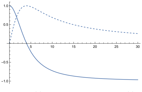
The paper claims that coupling the complex scalar field to a delta-function planar potential via $n_\mu j^\mu$, where $j^\mu$ is the Klein-Gordon current, produces a solvable quadratic theory whose Green function is exactly computable. The surprising consequences are that the potential exerts no force on a single stationary charge, that two charges interact as usual when on the same side of the plane, and that when they are on opposite sides the interaction energy is $$E_{\rm INT} = -\frac{1}{4\pi} Q_B^T \left[\frac{16-\$lambda^{2}$}{16+\$lambda^{2}$} I + \frac{8\$\lambda$}{16+\$lambda^{2}$} \tilde{I}\right] Q_C \frac{$e^{{-m|B-C|}}$}{|B-C|},$$ with $\tilde{I}$ the antisymmetric matrix that mixes the real and imaginary components of the charges. In the limit $\lambda\to\infty$ the matrix factor becomes $-I$, reversing the sign of the Yukawa interaction, and the field and its normal derivative vanish on the plane, yielding $j_3=0$. The paper also finds the energy remains finite when both charges lie on the plane, unlike typical delta-potential models, and that the differential operator in the field equations differs from the one in the Lagrangian.
Load-bearing premise
The load-bearing premise is that the products $\delta(x_3-a)\,\partial_3$ and $\partial_3\delta(x_3-a)$ are regulated with the convention $\operatorname{sgn}(0)=0$ and with discontinuous derivatives replaced by their average at the plane; if a different regularization is chosen, the Green function and the resulting interaction energies would change.
Editorial extensions
If this is right
- A single stationary scalar charge does not interact with the planar potential, which the paper identifies as the first field model where a spatially localized potential does not couple to a point charge.
- For two charges on opposite sides of the plane, the interaction energy is the Yukawa energy multiplied by the matrix $\frac{16-\lambda^2}{16+\lambda^2} I + \frac{8\lambda}{16+\lambda^2} \tilde{I}$, so the interaction can change sign for $\lambda>4$ and becomes a pure charge-mixing interaction at $\lambda=4$.
- When both charges are on the same side of the plane, the potential does not affect their interaction at all.
- When both charges lie on the plane itself, the interaction is the Yukawa interaction attenuated by the factor $16/(16+\lambda^2)$ and remains finite, in contrast with the divergences usually found when sources sit on delta-like potentials.
- In the $\lambda\to\infty$ limit, the Green function and the classical field satisfy Dirichlet and Neumann conditions on the plane, so the normal Klein-Gordon current $j_3$ vanishes there, giving a scalar analogue of the MIT boundary conditions.
Reading between the lines
- A natural extension the paper leaves implicit is to place two parallel such planes and use the exact Green function to compute the Casimir-like energy between them; the single-plane result would be the building block.
- The distributional products $\delta\,\partial_3$ and $\partial_3\delta$ are regulated with a specific averaging convention, so it is not known whether the $\lambda\to\infty$ MIT condition or the interaction matrix is stable under other self-adjoint extensions; checking symmetric versus asymmetric averaging would settle that.
- Because the energy (52) is not symmetric under exchanging the two charges, an observer on one side sees an effective charge rotated by the matrix in (55), while an observer on the other side sees a different effective charge; this direction-dependence could be probed in condensed-matter analogues using phonon or magnon fields.
- Replacing the delta function by a narrow smooth profile and taking the thin limit should reproduce equation (52) if the model is physically robust; deviations would indicate that the regularized delta prescription matters beyond the idealized plane.
Signed reviews
Editorial analysis
A structured set of objections, weighed in public.
Referee Report
Summary. The manuscript proposes a complex scalar field coupled to a delta-function planar potential through the normal Klein-Gordon current. Using a two-component matrix notation, the authors derive the field equation, obtain the Green function in a mixed Fourier representation, and compute the interaction energy of two stationary point charges. They report that a single charge does not interact with the plane, that charges on the same side interact through the ordinary Yukawa potential, and that charges on opposite sides experience a Yukawa interaction multiplied by a matrix factor α(λ)I + β(λ)I~. They also show that in the λ→∞ limit the field and its normal derivative vanish on the plane, giving j3=0 as a scalar analogue of the MIT boundary condition, and an appendix argues that the Hamiltonian is bounded from below.
Significance. The model is simple, exactly solvable at the Green-function level, and the closed-form interaction energy in Eq. (52) is a concrete, falsifiable prediction. The single-charge decoupling and the appearance of a λ-dependent mixing matrix are interesting and clearly presented. I have checked the reduction from Eq. (42) to Eq. (46) and the signs of the mixing terms in Eqs. (49), (50), and (52); these algebraic steps are internally consistent. The significance is, however, conditional: the exactness of the results depends on a distributional convention for the products δ∂3 and ∂3δ at the plane, and the paper does not state or justify that convention. If the authors can supply a well-defined regularization and show that the results are stable, the paper would be a valuable contribution; as it stands, the headline results are not uniquely defined.
major comments (2)
- [Section 2, Eqs. (11)-(12), (21), (27); Section 3.2.2, Eq. (57); Appendix Eq. (82)] The operator O(x)=λI~δ(x3−a)∂3+(λ/2)I~∂3δ(x3−a) contains products of distributions with fields that are discontinuous at the plane. The derivation fixes a convention through several unstated choices: integration by parts in Eq. (21) discards possible jump contributions, Eq. (27) sets sgn(0)=0, and Appendix Eq. (82) adopts the average of one-sided derivatives. These choices are not part of the Lagrangian (1) and are not shown to be the unique or physically preferred ones. For δ′ potentials in one dimension, different regularizations/self-adjoint extensions give different boundary conditions and different physics. The finite interaction energy for charges on the plane, Eq. (57), is a concrete example: it changes if sgn(0) is assigned a different value. Because Eq. (52) and the λ→∞ Dirichlet/Neumann/MIT limits are derived from this Green function, the central quantitative claims are not uniquely defined as stated. The authors should either specify a regularization or self-adjoint extension as part of the model definition and prove independence of admissible regularizations, or characterize how Eq. (52) changes under such choices.
- [Appendix A.2, Eqs. (78)-(83)] The proof that the Hamiltonian is bounded below assumes the eigenfunctions vs are continuous at z=a (the same amplitude A in Eq. (80)) and uses the averaging rule (82) for ∫δ v′ dz. For Schrödinger operators with δ′ potentials, self-adjoint boundary conditions generically include discontinuous eigenfunctions, so this ansatz does not exclude negative eigenvalues. The simplified model in Eq. (70) gives the condition λ²≤4m², whereas the appendix concludes boundedness for all λ; the discrepancy is not resolved. This matters because Section 2 invokes the appendix to assert the existence of a vacuum ground state at the quantum level.
minor comments (4)
- [Eq. (28)] The displayed coefficient 'λ2/m' in the Hamiltonian density is dimensionally inconsistent and does not match the single power of λ in the field equation (11); this appears to be a typo.
- [Eq. (26)] In the first line of Eq. (26), 'G0(p||;a,y3)' should read 'Gc0(p||;a,y3)' to be consistent with the notation used in the rest of the equation.
- [Conclusions, final paragraph before the Appendix] The sentence 'the mixing contribution ... varies within the interval [1, 0)' is inverted; β(λ)=8λ/(16+λ²) takes values in (0,1], with maximum 1 at λ=4.
- [Section 3.1 and Section 3.2.2] The vanishing of single-charge interaction and the finite on-plane interaction in Eq. (57) rely on the convention sgn(0)=0; this should be stated explicitly where the sign function is introduced, not only implicitly through Eq. (27).
Circularity Check
No significant circularity: the Green function, interaction energies, and λ→∞ limits are derived directly from the stated Lagrangian by explicit calculation.
full rationale
The paper's central results are self-contained derivations from the proposed Lagrangian (1). The Green function is obtained by solving the operator equation (13) through the integral equation (14), and the closed form (27) follows from algebraic manipulation of (21)–(26) with the free Green function (17). The interaction energies (35), (48), (49), and (52) are direct evaluations of the derived Green function with point-like sources; no parameter is fitted to a subset of results and no quantity called a prediction is equivalent to an input by construction. The λ→∞ Dirichlet, Neumann, and MIT-type conditions (60), (63), and (65) are limits of the explicitly computed Green function and its derivative, not assumptions imported from elsewhere. Self-citations in the reference list are contextual or methodological and are not load-bearing: no uniqueness theorem or prior result by the same authors is invoked to force the central claim. The appendix's distributional convention, e.g., Eq. (82), is an unproved regularization choice that may affect the model's definition, but that is a well-posedness/definitional caveat, not circular reasoning. The paper also explicitly leaves the boundary-condition formulation as an open question, further confirming that it does not rely on a self-citation chain for its main derivation.
Assumptions & free parameters
free parameters (1)
- lambda
assumptions (5)
- domain assumption Unique solution of the singular Green-function integral equation (14) and validity of the Fourier reduction in x||.
- domain assumption Distributional conventions at the plane: sgn(0)=0 and averaged one-sided derivatives in integrals of δ and δ' (Eq (82)).
- domain assumption External sources are stationary classical charges; self-energy divergences are discarded.
- domain assumption The differential operator D in Eq (73) is Hermitian and has a complete eigenbasis with real eigenvalues.
- standard math Standard Bessel-function integral identities (Gradshteyn-Ryzhik M0179a, Eq (45)) hold for m>0.
Cite this review
Pith. "Pith review of The role of scalar current coupling along surfaces." pith.science (2026). https://pith.science/paper/ETGHLPW4
@misc{pith2026250715625,
  author       = {Pith},
  title        = {Pith review of: The role of scalar current coupling along surfaces},
  year         = {2026},
  howpublished = {\url{https://pith.science/paper/ETGHLPW4}},
  note         = {Machine review of arXiv:2507.15625}
}
read the original abstract
In this paper we propose a coupling between the complex scalar field and an external Dirac delta-like planar potential. The coupling is achieved through the Klein-Gordon current normal to the plane where the potential is concentrated. The results are obtained exactly and exhibit many peculiarities. We show that a complex scalar charge does not interact with the potential, but the potential modifies the interaction between two scalar charges if they are placed on opposite sides of the planar potential. When the coupling constant between the potential and the field goes to infinity, the classical field solutions satisfy a kind of MIT boundary conditions along the plane where the potential is concentrated.
Figures

Reference graph
Works this paper leans on
-
[1]
K. A. Milton, The Casimir Effect, Physical Manifestations of Zero-Point Energy (World Scientific, Singapore, 2001)
work page 2001
-
[2]
M. Bordag, U. Mohideen, and V. M. Mostepanenko, Phys. Rep. 353, 1 (2001). https://doi.org/10.1016/S0370-1573%2801%2900015-1
-
[3]
M. Bordag and J. M. Mu˜ noz-Casta˜ neda, Phys. Rev. D91, 065027 (2015). https://doi.org/10.1103/PhysRevD.91.065027 20
-
[4]
J.M. Mu˜ noz-Casta˜ neda, J.M. Guilarte and A.M. Mosquera, Phys. Rev. D87, 105020 (2013). https://doi.org/10.1103/PhysRevD.87.105020
-
[5]
F.A. Barone and F.E. Barone, Phys. Rev. D 89, 065020 (2014). https://doi.org/10.1103/PhysRevD.89.065020
-
[6]
F.A. Barone and F.E. Barone, Eur. Phys. J. C 74, 3113 (2014). https://doi.org/10.1140/epjc/s10052-014-3113-y
-
[7]
N. Graham, R. L. Jaffe, V. Khemani, M. Quandt, M. Scandurra and H. Weigel, Nucl. Phys. B 645, 49 (2002). https://doi.org/10.1016/S0550-3213%2802%2900823-4
-
[8]
M. Bordag, D. Hennig, and D. Robaschik, J. Phys. A 25, 4483 (1992). https://doi.org/10.1088/0305-4470/25/16/023
Show all 52 references
-
[9]
Milton, J
Kimball A. Milton, J. Phys. A 37, 6391 (2004). https://doi.org/10.1088/0305-4470/37/24/014
2004 doi
- [10]
-
[11]
Camilo, F.A
G.T. Camilo, F.A. Barone and F.E. Barone, Phys. Rev. D 87 025011 (2013). https://doi.org/10.1103/PhysRevD.87.025011
2013 doi
-
[12]
Shajesh, P
K.V. Shajesh, P. Parashar, I. Brevik, Ann. Phys. 387, 166 (2017). https://doi.org/10.1016/j.aop.2017.10.008
2017 doi
-
[13]
Bordag and I.G
M. Bordag and I.G. Pirozhenko, Phys. Rev. D 95, 056017 (2017). https://doi.org/10.1103/PhysRevD.95.056017
2017 doi
-
[14]
Bordag, Phys
M. Bordag, Phys. Rev. D 89, 125015 (2014). https://doi.org/10.1103/PhysRevD.89.125015
2014 doi
-
[15]
Milton, P
K.A. Milton, P. Kalauni, P. Parashar and Y. Li, Phys. Rev. D 96, 085007 (2017). https://doi.org/10.1103/PhysRevD.96.085007
2017 doi
-
[16]
Milton, P
K.A. Milton, P. Kalauni, P. Parashar and Yang Li, Phys. Rev. D 99, 045013 (2019). https://doi.org/10.1103/PhysRevD.99.045013 21
2019 doi
-
[17]
Parashar, K.A
P. Parashar, K.A. Milton, K.V. Shajesh and Iver Brevik, Phys. Rev. D 96, 085010 (2017). https://doi.org/10.1103/PhysRevD.96.085010
2017 doi
-
[18]
Bordag, K
M. Bordag, K. Kirsten, and D. Vassilevich, Phys. Rev. D 59, 085011 (1999). https://doi.org/10.1103/PhysRevD.59.085011
1999 doi
-
[19]
Mu˜ noz-Casta˜ neda and J.M
J.M. Mu˜ noz-Casta˜ neda and J.M. Guilarte, Phys. Rev. D91, 025028 (2015). https://doi.org/10.1103/PhysRevD.91.025028
2015 doi
-
[20]
Braga, J.D.L
A.N. Braga, J.D.L. Silva and D.T. Alves, Phys. Rev. D 94, 125007 (2016). https://doi.org/10.1103/PhysRevD.94.125007
2016 doi
-
[21]
Milton, P
Yang Li, K.A. Milton, P. Kalauni and P. Parashar, Phys. Rev. D 94, 085010 (2016). https://doi.org/10.1103/PhysRevD.94.085010
2016 doi
-
[22]
Milton, Y
K.A. Milton, Y. Li, P. Kalauni, P. Parashar, R. Gu´ erout, Gert-Ludwig Ingold, A. Lambrecht and S. Reynaud, Fortschr. Phys. 65, 1600047 (2017). https://doi.org/10.1002/prop.201600047
2017 doi
-
[23]
Venkat Abhignan, Phys. Scr. 98 105018 (2023). https://doi.org/10.1088/1402-4896/acee2c
2023 doi
-
[24]
Milton, P
K.A. Milton, P. Parashar, M. Schaden and K.V. Shajesh, Nuovo Cim. 36 C, 193 (2013). https://doi.org/10.1393/ncc/i2013-11532-4
2013 doi
-
[25]
Parashar, K.A
P. Parashar, K.A. Milton, K.V. Shajesh and M. Schaden, Phys. Rev. D 86, 085021 (2012). https://doi.org/10.1103/PhysRevD.86.085021
2012 doi
-
[26]
Oliveira, L.H.C
H.L. Oliveira, L.H.C. Borges, F.E. Barone, F.A. Barone, Eur. Phys. J. C 81, 558 (2021). https://doi.org/10.1140/epjc/s10052-021-09356-6
2021 doi
-
[27]
Santamar ´ ıa-Sanz, J
L. Santamar ´ ıa-Sanz, J. Phys. A: Math. Theor.56 385201 (2023). https://doi.org/10.1088/1751-8121/acef0d
2023 doi
-
[28]
Sundberg, R.L
P. Sundberg, R.L. Jaffe, Ann. Phys. 309, 442 (2004). https://doi.org/10.1016/j.aop.2003.08.015
2004 doi
-
[29]
Adamyan, B.S Pavlov, J Math
V.M. Adamyan, B.S Pavlov, J Math. Sci. 42, 1537 (1988). https://doi.org/10.1007/BF01665040 22
1988 doi
-
[30]
Demkov and V
Y.N. Demkov and V. Ostrovsky, Zero-Range Potentials and Their Applications in Atomic Physics , Plenum Press, New York, (1988)
1988
-
[31]
Kulinskii and D.Y
V.L. Kulinskii and D.Y. Panchenko, Front. Phys. 7, 44 (2019). https://doi.org/10.3389/fphy.2019.00044
2019
-
[32]
Albeverio, F
S. Albeverio, F. Gesztesy, R. Hoegh-Krohn and H. Holden, with an appendix by Pavel Exner, Solvable Models in Quantum Mechanics , 2nded., AMS Chelsea Publishing vol. 350, Providence, Rhode Island, USA, (2005)
2005
-
[33]
Schmidt, B.K
A.G.M. Schmidt, B.K. Cheng and M.G.E. da Luz, Phys. Rev. A 66, 062712 (2002). https://doi.org/10.1103/PhysRevA.66.062712
2002 doi
-
[34]
Carreau, J
M. Carreau, J. Phys.: Math. General 26, 427 (1993). https://doi.org/10.1088/0305-4470/26/2/025
1993 doi
-
[35]
Albeverio and P
S. Albeverio and P. Kurasov, Singular Perturbations of Differential Operators. Solvable Schr¨ odinger Type Operators, London Mathematical Society, Lecture Note Series vol. 221, Cambridge University Press, Cambridge (2000)
2000
-
[36]
Griffiths and D.F
D.J. Griffiths and D.F. Schroeter, Introduction to quantum mechanics, 3rd ed., Cambridge University Press (2018)
2018
-
[37]
Deser, R
S. Deser, R. Jackiw and S. Templeton, Ann. Phys. (NY) 140, 372 (1982). https://doi.org/10.1016/0003-4916(82)90164-6
1982 doi
-
[38]
Helay¨ el-Neto, M.A
J.A. Helay¨ el-Neto, M.A. Santos and I.V. Vanceac, Braz. J. Phys. 36, 1305 (2006). https://doi.org/10.1590/S0103-97332006000700033
2006 doi
-
[39]
de Oliveira, Rev
D.M. de Oliveira, Rev. Bras. Ens. Fis., 33, 3309 (2011). https://doi.org/10.1590/S1806-11172011000300009
2011 doi
-
[40]
Cremmer and J
E. Cremmer and J. Scherk, Nucl. Phys. B 72, 117 (1974). https://doi.org/10.1016/0550-3213(74)90224-7
1974 doi
-
[41]
Allen, M.J
T.J. Allen, M.J. Bowick and A. Lahiri, Mod. Phys. Lett. A 6, 559 (1991). https://doi.org/10.1142/S0217732391000580
1991 doi
-
[42]
Barone, F.E
F.A. Barone, F.E. Barone and J. A. Helay¨ el-Neto, Phys. Rev. D 84, 065026 (2011). https://doi.org/10.1103/PhysRevD.84.065026 23
2011 doi
-
[43]
Carroll, G.B
S.M. Carroll, G.B. Field and R. Jackiw, Phys. Rev. D 41, 1231 (1990). https://doi.org/10.1103/PhysRevD.41.1231
1990 doi
-
[44]
Adam and F.R
C. Adam and F.R. Klinkhamer, Nucl. Phys. B 607, 247 (2001). https://doi.org/10.1016/S0550-3213(01)00161-4
2001 doi
-
[45]
Adam and F.R
C. Adam and F.R. Klinkhamer, Nucl. Phys. B 657, 214 (2003). https://doi.org/10.1016/S0550-3213(03)00143-3
2003 doi
-
[46]
Belich, M.M
H. Belich, M.M. Ferreira Jr, J.A. Helay¨ el-Neto, M.T.D. Orlando, Phys. Rev. D 67, 125011 (2003); -ibid, Phys. Rev. D 69, 109903 (E) (2004). https://doi.org/10.1103/PhysRevD.67.125011 https://doi.org/10.1103/PhysRevD.69.109903
2003 doi
-
[47]
Belich, M
H. Belich, M. M. Ferreira Jr, J.A. Helay¨ el-Neto, M.T.D. Orlando, Phys. Rev. D 68, 025005 (2003). https://doi.org/10.1103/PhysRevD.68.025005
2003 doi
-
[48]
Belich, M
H. Belich, M. M. Ferreira Jr and J. A. Helay¨ el-Neto, Eur. Phys. J. C 38, 511 (2005). https://doi.org/10.1140/epjc/s2004-02033-x
2005 doi
-
[49]
Belich, T
H. Belich, T. Costa-Soares, M.M. Ferreira Jr., J.A. Helay¨ el-Neto, Eur. Phys. J. C 42, 127 (2005). https://doi.org/10.1140/epjc/s2005-02253-6
2005 doi
-
[50]
Chodos, R.L
A. Chodos, R.L. Jaffe, K. Johnson, C.B. Thorn, V.F. Weisskopf, Phys. Rev. D 9, 3471 (1974). https://doi.org/10.1103/PhysRevD.9.3471
1974 doi
-
[51]
Gradshteyn and I.M
I.S. Gradshteyn and I.M. Ryzhik, Table of Integrals, Series and Products , 7 thed., Academic Press, USA (2007)
2007
-
[52]
Flores-Hidalgo et al
G. Flores-Hidalgo et al. , work in progress. 24
Reviewed August 6, 2026 · model on record in the stance chip above.
Discussion (0). Continue with ORCID to comment.