REVIEW 3 major objections 6 minor 1 cited by
Sampler-free gravitational wave inference using matrix multiplication
T0 review · 3 major / 6 minor · reviewed 2026-08-06 · deepseek-v4-flash
Pith's one-line read Bayesian gravitational-wave inference can be done by matrix multiplication, in minutes on one CPU.
desk verdict Genuinely fast sampler-free PE with real validation, but the headline accuracy is benchmarked only against a denser version of itself and the bank-edge truncation risk is untested. read the letter →
The pith
A machine-rendered reading of the paper's core claim, the machinery that carries it, and where it could break.
The reading
What carries the argument
The load-bearing object is the sum-of-products decomposition of the likelihood: each mode-polarization-detector-frequency contribution separates into a factor of intrinsic parameters, a factor of extrinsic parameters, and a phase factor, so that the inner products $\langle d|h\rangle$ and $\langle h|h\rangle$ are assembled by tensor contractions instead of per-point waveform generation. Relative binning reduces each waveform to about 378 coarse frequency points while retaining better than 1% log-likelihood accuracy. A precomputed intrinsic bank organized by chirp mass (the mass combination that sets the signal's frequency sweep), an incoherent maximum-likelihood cut, and adaptive importance sampling of the extrinsic parameters provide the discrete grid over which the matrix products run, while distance is marginalized through the closed-form likelihood form.
What would settle it
Generate an injection whose chirp mass sits just outside the edge of the chosen bank at a signal-to-noise ratio of 8, run the method, and compare the reported log evidence with a dense reference integral over the full prior; if the error systematically exceeds the claimed ±1 in log evidence, the bank-coverage assumption is falsified.
Extended reading notes
Core claim
The central claim is that the full Bayesian evidence and posterior for a precessing, higher-mode compact binary coalescence can be obtained by evaluating a stored intrinsic waveform bank against an importance-sampled extrinsic set using matrix products, with the distance marginalization done analytically. The likelihood decomposes so that inner products factor by frequency bin, azimuthal mode, polarization, and detector; summing these factors with a matrix contraction gives the likelihood for all intrinsic-extrinsic-reference-phase combinations at once. After an incoherent preselection removes waveforms that cannot match the data, the evidence is the weighted average of the distance-marginalized likelihoods over the product set. The paper validates the procedure on 1,024 synthetic signals per mass range, with median log-evidence errors near 0.5 and upper quartiles near 1.1, and shows that the resulting posterior samples agree with a stochastic-sampler reference on example events.
Load-bearing premise
The evidence integral is only as correct as the precomputed bank's coverage: the bank's mass range is set by an empirical, by-eye scaling of the 90% confidence intervals of 93 previously detected events, scaled to a signal-to-noise ratio of 8, so a real trigger whose posterior support extends beyond that range would get a biased evidence and posterior.
Editorial extensions
If this is right
- The evidence ratio, the optimal detection statistic, becomes cheap enough to compute for every matched-filter trigger, so searches can include precession and higher modes without a separate expensive sampling stage.
- Posterior samples, and thus parameter estimates and sky localization, are available in minutes for a single event, making electromagnetic follow-up faster.
- Because waveforms are generated once and stored, the online cost no longer depends on how expensive the waveform model is; more accurate models can be dropped into the same bank framework.
- The relation between sample counts and integration error is quantified, so run settings can be chosen ahead of time to meet a target log-evidence accuracy.
- The posterior weights can be reweighted to different priors in post-processing, so one bank run per event can serve multiple population analyses.
Reading between the lines
- One caution not developed in the paper: bank coverage is calibrated to previously observed events, so the first strong event with unusual mass or spin properties could have posterior support outside the bank; a coverage diagnostic built from the stated effective-sample-size checks would be a prudent addition before trusting evidence values in a real search.
- The matrix-product core is trivially parallel and GPU-friendly, so the same algorithm should reach seconds-per-event on accelerator hardware, making full evidence-based follow-up of all current-era triggers practical in real time.
- The same factorization strategy should transfer to other signal families, such as eccentric binaries or tidal waveforms, provided their likelihoods admit a similar sum-of-products separation; a testable extension would be to build a coarse bank for eccentric signals and check convergence.
- The factorization assumes static antenna responses, which the paper notes breaks down for next-generation detectors with longer in-band signals; extending the method there would require time-dependent antenna-response blocks inside the matrix products.
Editorial analysis
A structured set of objections, weighed in public.
Referee Report
Summary. The manuscript presents dot-PE, a sampler-free Bayesian parameter-estimation method for precessing compact-binary coalescence signals with higher-order modes. The likelihood is decomposed into intrinsic, extrinsic, reference-phase, and distance components, so that the distance-marginalized likelihood can be evaluated for all combinations of precomputed intrinsic waveforms, adaptively importance-sampled extrinsic parameters, and phase-grid points through matrix multiplications. The Bayesian evidence is then computed as a weighted sum over this Cartesian product. The authors report an accuracy of approximately ±1 in ln Z within minutes on a single CPU core, validate the method with 1,024 injections per six chirp-mass ranges, show P-P calibration plots, and compare posterior samples with cogwheel/nautilus for three synthetic events. The central concern is that the evidence integral is restricted to a precomputed chirp-mass bank whose bounds are set by an empirical, by-eye scaling relation, and the accuracy benchmarks compare against a denser version of the same finite-bank pipeline.
Significance. If the accuracy claim holds, the method is practically significant: it offers a fast, predictable, and parallelizable alternative to stochastic samplers for CBC parameter estimation, including higher modes and precession, and it enables evidence-based search follow-up. The paper's strengths include the clean likelihood decomposition, the use of precomputed waveform banks that avoid online waveform generation, a public code repository, and extensive injection-based testing with P-P plots and nested-sampling comparisons on three events. However, the headline accuracy is currently established only relative to a denser version of the same method with the same finite chirp-mass bounds, so the bank-support question is load-bearing and must be addressed before the central claim can be considered fully validated.
major comments (3)
- [Sec. 4.3, Eq. (40), Fig. 2] The evidence integral in Eq. (40) is a weighted sum over the precomputed intrinsic bank, so the chirp-mass bounds of Sec. 4.3 (Fig. 3) act as part of the effective prior. If a real trigger's posterior extends beyond or lies near the edge of the assigned bank, the evidence is biased low and the posterior is truncated. This error is invisible in Fig. 2 because the reference runs use the same bank bounds with a denser bank (N_int = 2^18), not an independent method. The by-eye power-law fit to GWTC-3 90% confidence intervals scaled to SNR 8 is not validated for triggers outside that population (e.g., lower SNR, extreme mass ratio, different detector PSD, or stronger precession/higher-mode content). Please add explicit edge-coverage tests, including injections near or outside the nominal bank bounds, and an absolute evidence check against an independent sampler with a wide chirp-mass prior.
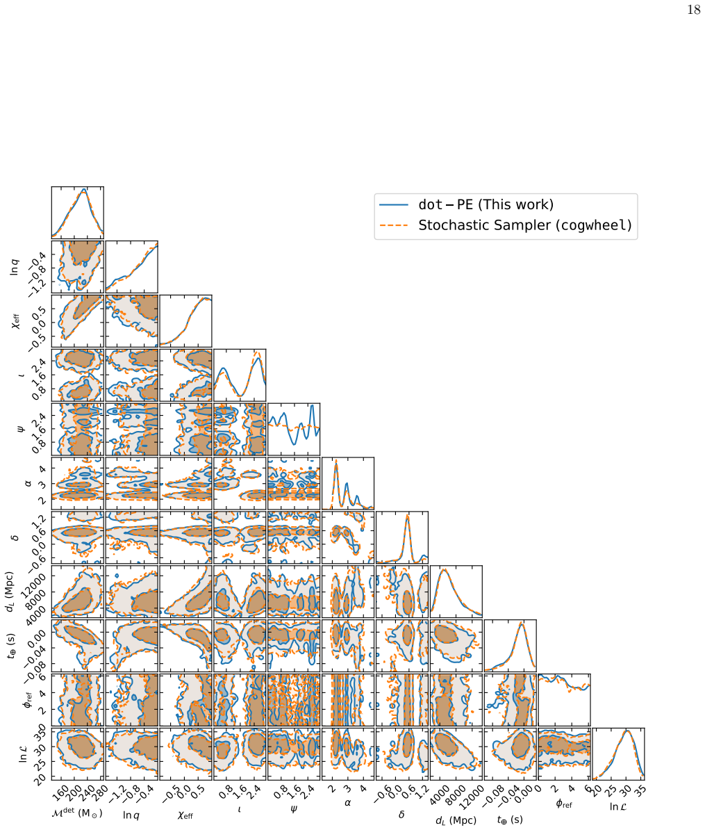
- [Sec. 5.2, Figs. 7-9] The three comparison runs with cogwheel/nautilus are limited to the same M and q ranges as the banks ('We limit cogwheel's M and q to the same ranges as the used intrinsic sample banks'), and they test posterior agreement rather than the evidence Z. As a result, they cannot validate the headline ±1 in ln Z accuracy or the adequacy of the bank support. Please report the log-evidence differences for these three events against the external sampler, and run at least one comparison with a deliberately broader chirp-mass prior, or with an injection placed near the bank edge, so that bank truncation would show up as a discrepancy.
- [Sec. 5, Fig. 6] The P-P plots exclude runs that produced fewer than 30 posterior samples, as indicated by the titles (e.g., N = 911/1024 to 1019/1024). The calibration statement is therefore conditional on successful runs. If the excluded events preferentially lie near the bank edges or at low SNR, the P-P curves would overstate coverage. Please report the distribution of excluded events in chirp mass, mass ratio, and SNR, or repeat the calibration after including them.
minor comments (6)
- [Sec. 4.2, Eq. (38)] In Eq. (38), the left-hand side is written as 'ln L_ieo' but the right-hand side is the distance-marginalized likelihood, not its logarithm; the notation should be corrected to L_ieo.
- [Abstract and Sec. 2] The phrase 'without relying on stochastic samplers' is somewhat overstated, because the extrinsic-parameter proposal uses random importance sampling; a more precise wording would be 'without MCMC or nested sampling'.
- [Sec. 4.3, Fig. 3] The bank chirp-mass scaling is described as 'calibrated by-eye'; because these bounds are load-bearing for the evidence integral, the fitted prefactor and power-law exponent should be stated explicitly or provided in a reproducibility table.
- [Appendix B, Eq. (45)] The sentence 'Summing the likelihoods independently maximized in different detectors' is misleading: Eq. (45) sums the separately maximized log-likelihoods, not the likelihoods themselves.
- [Sec. 5.1, Eq. (56)] The notation in Eq. (56) uses N_int on both sides of the approximation, which is confusing; the left-hand side should be labeled as the number of bank samples within the chirp-mass confidence interval, e.g., N_int^CI.
- [Table I caption] The sentence 'Subscripts and superscripts stand for 0.25 and 0.75 quantile' is unclear; the caption should explicitly state that the central value is the median and the sub/superscripts are the 25th and 75th percentiles.
Circularity Check
The ±1 ln Z accuracy claim is benchmarked against a denser version of the same method sharing the same fitted chirp-mass support: the bank M-bounds are a by-eye fit to GWTC-3 90% CIs, so support truncation is invisible to every validation channel, including the nested-sampling comparisons.
-
other
[Sec. 4.3 (Eq. 40); Fig. 2 caption; Sec. 5.1 (Eq. 56)]
"Reference values Ẑ are computed with much finer banks of N int = 2 18 ≈2.6×10 5. ... The relevant confidence intervals of M are determined from the same injection runs analyzed throughout this section. ... The prefactor and power-law are calibrated by-eye using the posterior samples of the 93 GWTC-3 events [5], as presented in Fig. 3."
Eq. (40) evaluates Z as a weighted sum over the precomputed intrinsic bank only, so the integral's correctness depends entirely on that bank covering the posterior support. In Fig. 2 and Table I, the reference Ẑ is the same integral evaluated with a denser bank (N_int = 2^18) but over the same chirp-mass bounds, whose width is a by-eye power-law fit to the 90% CIs of the 93 GWTC-3 events (Sec. 4.3). Both the estimate and the reference therefore share the identical support truncation; the measured |ln Z − ln Ẑ| isolates only sample-density and weight-convergence error. Any bias from posterior mass falling outside the fitted M-range cancels by construction, and since the CI widths used to build the banks (Eq.
-
other
[Sec. 5.2]
"We limit cogwheel’s M and q to the same ranges as the used intrinsic sample banks."
The only external-ground-truth comparisons in the paper (nested sampling via cogwheel/nautilus, Figs. 7–9) impose the same truncated M-prior as the bank under test. Agreement with the external sampler therefore verifies the in-support computation (grid density, importance weights, pre-selection, distance marginalization) but cannot, by construction, detect whether the fitted bank support is complete. This makes the one independent validation channel consistent with the self-referential dense-bank benchmark rather than checking the same truncation risk; the completeness of the fitted support remains asserted on the strength of the Sec. 4.3 by-eye calibration alone.
full rationale
The core evidence computation is not construction-level circular: Eq. (40)/Eq. (3) is an honest importance-sampled sum of distance-marginalized likelihoods obtained from the data and a waveform model, and the posterior P–P tests (Fig. 6) use independent injections drawn from the stated priors, so the sampling machinery is genuinely exercised. The three nested-sampling comparisons (Figs. 7–9) are real external checks of the in-support posterior and show agreement. What keeps this from a clean 0–2 score is that the central accuracy claim is validated only through a chain that shares its own inputs: the bank chirp-mass bounds are fitted by eye to the 90% CIs of the 93 GWTC-3 events (Sec. 4.3), the Fig. 2/Table I reference values are denser versions of the same integral over the same bounds, the CI widths used for predicting acceptance rates come from the same injection runs (Eq. 56), and the external nested-sampling runs restrict their priors to the same bank ranges (Sec. 5.2). Hence a systematic truncation bias is invisible to every validation channel, making the ±1 ln Z claim conditional on the fitted support rather than independently established. This is partial circularity of the benchmark and of the fitted input, not a derivation equivalent to its inputs: the evidence numbers themselves are not forced by the fit. The load-bearing imports from the authors' own prior work (relative binning [17,27]; cogwheel distance marginalization and adaptive importance sampling [25]) are code-reproduced, summarized in Appendices A–C, and cross-checked against nautilus, so they are real evidence and do not by themselves raise the score. Overall score 4: some self-reference in the validation and a fitted support limitation, while the central algorithmic claim retains independent content.
Assumptions & free parameters
free parameters (7)
- Bank mass-range scaling prefactor and power-law exponent =
Not given numerically; drawn by eye as the black line in Fig. 3
- Delta ln L_ML cutoff in Eq. (39) =
20
- Delta L_inco.ML cutoff in Eq. (45) =
20
- N_c = 16 intrinsic samples for extrinsic proposal aggregation =
16
- Proposal acceptance thresholds =
N_eff >= 100 and N_eff_prior >= 50
- Inverse temperature beta in arrival-time proposal =
~0.5
- Relative-binning frequency points N_f =
378
assumptions (6)
- domain assumption Noise hypothesis H0: detector data is stationary Gaussian noise with known power spectral density.
- domain assumption The waveform decomposition in Eq. (28) assumes the detector response F_kp and time-shift T_k are constant over the signal duration in the sensitive band.
- domain assumption Signals are quasi-circular, non-eccentric, non-tidal compact binary coalescences described by the IMRPhenomXODE waveform model.
- standard math Relative binning with 378 frequency points yields log-likelihood accuracy better than 1%.
- domain assumption The extrinsic importance sampling method of [25] is correct and yields unbiased proposals when aggregated over N_c intrinsic samples.
- domain assumption The incoherent per-detector maximum likelihood is a sufficient proxy for selecting intrinsic waveforms that can contribute to the coherent evidence.
Cite this review
Pith. "Pith review of Sampler-free gravitational wave inference using matrix multiplication." pith.science (2026). https://pith.science/paper/4PCXYMDQ
@misc{pith2026250716022,
  author       = {Pith},
  title        = {Pith review of: Sampler-free gravitational wave inference using matrix multiplication},
  year         = {2026},
  howpublished = {\url{https://pith.science/paper/4PCXYMDQ}},
  note         = {Machine review of arXiv:2507.16022}
}
abstract
Parameter estimation (PE) for compact binary coalescence (CBC) events observed by gravitational wave (GW) laser interferometers is a core task in GW astrophysics. We present a method to compute the posterior distribution efficiently without relying on stochastic samplers. First, we show how to select sets of intrinsic and extrinsic parameters that efficiently cover the relevant phase space. We then show how to compute the likelihood for all combinations of these parameters using dot products. We describe how to assess and tune the integration accuracy, making the outcome predictable and adaptable to different applications. The low computational cost allows full PE in minutes on a single CPU, with the potential for further acceleration using multiple CPUs or GPUs. We implement this method in the $\texttt{dot-PE}$ package, enabling sensitive searches using the full evidence integral for precessing CBCs and supporting large waveform banks ($\sim10^5$--$10^6$ waveforms), regardless of waveform generation cost.
Figures


Figures from the paper (6 more)


Forward citations
Cited by 1 Pith paper
-
Improving low-latency multi-messenger follow-up of neutron star-black hole mergers with mode-by-mode filtering
Mode-by-mode filtering of higher-order modes enables low-latency marginalization over mode information in NSBH gravitational-wave signals, tightening constraints on distance, inclination, and secondary mass.
Reference graph
Works this paper leans on
-
[1]
The intricate informa- tion about the masses of the compact objects and their spin vectors is encoded in the fine details of the received gravitational waves
INTRODUCTION Compact objects (neutron stars and black holes) in binaries undergoing mergers emit gravitational waves (GW), and are being frequently detected by ground- based laser interferometers [1, 2]. The intricate informa- tion about the masses of the compact objects and their spin vectors is encoded in the fine details of the received gravitational w...
2025
-
[2]
A block diagram of our method is presented in Fig
SUMMAR Y OF THIS WORK In this work, we propose a new scheme for the Bayesian inference problem of CBC using GW interferometer data, including the effects of higher modes and precession. A block diagram of our method is presented in Fig. 1. The waveform, and therefore also the likelihood, can be writ- ten as a sum-of-products of components, that depend on ...
arXiv 2025
-
[3]
The pipeline trigger provides a rough estimate of the chirp mass, which lets us restrict the intrinsic samples to the corresponding pre-computed set of waveforms (see Sec. 4.3). For example, while the full parameter space may cover chirp masses from 3 to 300 M ⊙, a trigger of a template with chirp mass near 25 M ⊙ allows us to focus on the much narrower r...
-
[4]
Given the data, we include or exclude each of theN int. intrinsic waveforms according to a likeli- hood maximizedincoherentlyacross detectors (i.e., the maximization overθ ext,ϕ ref , andd L is done per detector, without cross-detector consistency). This pre-selection retainsN ′ int. intrinsic samples (Sec. 4.4)
-
[5]
Given a random selection of intrinsic samples, we employ an adaptive importance sampling method
-
[6]
CONCLUSIONS We have presented a novel approach to the posterior estimation problem of CBC GW events. We split the 15 dimensions of parameter space into 4 subsets, accord- ing to their functional form in the likelihood function. This allows us to evaluate the (distance-marginalized) likelihood for each intrinsic-extrinsic-phase combination, using a sequenc...
work page 2023
-
[7]
Detection: The main motivation is to compute Z, which is the optimal test statistic for a search [32], quickly and reliably, as a second stage after a matched-filtering pipeline. 3
-
[8]
Parameter estimation: Detected events are ana- lyzed by drawing samples from the posterior dis- tribution of the source parameters, defined by the probabilistic weights in Eq. (3). By modifying the weightswin post-processing, we can also resample from different priors
Show all 83 references
-
[9]
The individual maximum-likelihood point can be used for fitting and signal consistency checks [33]
-
[10]
Fast sampling from the posterior can be used for quick sky-localization, which is useful of electro- magnetic followup. The method presented here carries two important advan- tages with respect to traditional sampling methods: •There is little-to-no online waveform generation ...
-
[11]
The review is not exhaustive, and limits the discussion to what is rele- vant in this work, in addition to the current community- standard in the field of parameter estimation
PRELIMINARIES In this section we will review the basics for Bayesian inference and integration of the evidence. The review is not exhaustive, and limits the discussion to what is rele- vant in this work, in addition to the current community- standard in the field of parameter ...
-
[12]
W aveform Decomposition The imprint of the gravitational waves from CBC sources into the strain at the detector depends on 15 pa- rameters
METHOD 4.1. W aveform Decomposition The imprint of the gravitational waves from CBC sources into the strain at the detector depends on 15 pa- rameters. We limit to discussion to quasi-circular (zero eccentricity) binaries without tidal deformability. We separate the parameters...
-
[13]
1,024 injections are performed for each of 6 chirp mass ranges: (3,3.2)M ⊙, (5,5.6)M ⊙, (10,12)M ⊙, (20,30)M ⊙, (50,100)M ⊙, and (100,300)M ⊙
PERFORMANCE We test the performance of our method against injec- tions into synthetic noise realizations, using the Hanford– Livingston–Virgo detector network with O3 sensitivities. 1,024 injections are performed for each of 6 chirp mass ranges: (3,3.2)M ⊙, (5,5.6)M ⊙, (10,12)...
-
[14]
B. Farr, E. Ochsner, W. M. Farr, and R. O’Shaughnessy, Phys. Rev. D90, 024018 (2014), arXiv:1404.7070 [gr-qc]
2014 arXiv
-
[15]
The effective sample size is evaluated both with and without the likelihood
-
[16]
The proposalsπ ′ fromN c = 16 different intrinsic samples are drawn, to decouple between the intrin- sic and extrinsic samples (mainly due to inclination correlations with sky positions, [59, 60])
-
[17]
Overhead
The extrinsic samples are drawn uniformly, and the prior-ratio is taken as the importance-sampling weightsw e. Appendix D: Complexity and runtime To test the runtime of the code in realistic settings, we choseN int. andN ext. per intrinsic sample bank based on the results of S...
-
[18]
LIGO Scientific Collaboration, J. Aasi, B. P. Abbott, R. Abbott,et al., Classical and Quantum Gravity32, 074001 (2015), arXiv:1411.4547 [gr-qc]
2015 arXiv
-
[19]
Aasiet al., Classical and Quantum Gravity29, 155002 (2012)
J. Aasiet al., Classical and Quantum Gravity29, 155002 (2012)
2012
-
[20]
Abbott, H
R. Abbott, H. Abe, F. Acernese, K. Ackley,et al., The Astrophysical Journal Supplement Series267, 29 (2023), arXiv:2302.03676 [gr-qc]
2023 arXiv
-
[21]
New black hole mergers in the LIGO–Virgo O3 data from a gravitational wave search including higher- order harmonics,
D. Wadekar, J. Roulet, T. Venumadhav, A. K. Mehta, et al., “New black hole mergers in the LIGO–Virgo O3 data from a gravitational wave search including higher- order harmonics,” (2023), arXiv:2312.06631 [gr-qc]
2023 arXiv
-
[22]
Abbottet al.(LIGO Scientific Collaboration, Virgo Collaboration, and KAGRA Collaboration), Phys
R. Abbottet al.(LIGO Scientific Collaboration, Virgo Collaboration, and KAGRA Collaboration), Phys. Rev. X13, 041039 (2023)
2023
-
[23]
A. H. Nitz, S. Kumar, Y.-F. Wang, S. Kastha,et al., Astrophys. J.946, 59 (2023), arXiv:2112.06878 [astro- ph.HE]
2023 arXiv
-
[24]
Capote, W
E. Capote, W. Jia, N. Aritomi, M. Nakano,et al., Phys. Rev. D111, 062002 (2025), arXiv:2411.14607 [gr-qc]
2025 arXiv
-
[25]
After the phase space narrowing stage, the parameter space is represented by the Cartesian product of the three selected sets: n θ(i) int oN ′ int
to draw extrinsic parameters that are consis- tent with the arrival times at the different detec- tors. After the phase space narrowing stage, the parameter space is represented by the Cartesian product of the three selected sets: n θ(i) int oN ′ int. i=1 , n θ(e) ext oNext. e...
-
[26]
LIGO detects 200th gravitational- wave candidate in O4,
LIGO Laboratory, “LIGO detects 200th gravitational- wave candidate in O4,”https://www.ligo.caltech. edu/MIT/news/ligo20250320(2025), accessed: 2025-06- 05
2025
-
[27]
A. Abac, R. Abramo, S. Albanesi, A. Albertini, A. Agapito, M. Agathos,et al., arXiv e-prints , arXiv:2503.12263 (2025), arXiv:2503.12263 [gr-qc]
2025 arXiv
-
[28]
Evans, R
M. Evans, R. X. Adhikari, C. Afle, S. W. Ballmer, et al., arXiv e-prints , arXiv:2109.09882 (2021), arXiv:2109.09882 [astro-ph.IM]
2021 arXiv
-
[29]
LIGO Scientific Collaboration,Report from the LSC Post-O5 Study Group, Tech. Rep. LIGO-T2200287–v3 (LIGO Document Control Center, 2024)
2024
-
[30]
Saleem, J
M. Saleem, J. Rana, V. Gayathri, A. Vijaykumar, et al., Classical and Quantum Gravity39, 025004 (2022), arXiv:2105.01716 [gr-qc]
2022 arXiv
-
[31]
Marginalisation of the time and phase parame- ters in CBC parameter estimation,
W. Farr, “Marginalisation of the time and phase parame- ters in CBC parameter estimation,”https://dcc.ligo. org/public/0114/T1400460/002/margtime.pdf(2014)
2014
-
[32]
Veitch, V
J. Veitch, V. Raymond, B. Farr, W. Farr,et al., Physical Review D91(2015), 10.1103/physrevd.91.042003
2015 doi
-
[33]
Pankow, P
C. Pankow, P. Brady, E. Ochsner, and R. O’Shaughnessy, Physical Review D92(2015), 10.1103/physrevd.92.023002
2015 doi
-
[34]
Relative bin- ning and fast likelihood evaluation for gravitational wave parameter estimation,
B. Zackay, L. Dai, and T. Venumadhav, “Relative bin- ning and fast likelihood evaluation for gravitational wave parameter estimation,” (2018), arXiv:1806.08792 [astro- ph.IM]
2018 arXiv
-
[35]
C. M. Biwer, C. D. Capano, S. De, M. Cabero, D. A. Brown, A. H. Nitz, and V. Raymond, Publications of the Astronomical Society of the Pacific131, 024503 (2019)
2019
-
[36]
M. Dax, S. R. Green, J. Gair, J. H. Macke, A. Buonanno, and B. Sch¨ olkopf, Phys. Rev. Lett.127, 241103 (2021)
2021
-
[37]
Gabbard, C
H. Gabbard, C. Messenger, I. S. Heng, F. Tonolini, and R. Murray-Smith, Nature Physics18, 112–117 (2021)
2021
-
[38]
Factorized parameter estimation for real-time gravitational wave in- ference,
T. Islam, J. Roulet, and T. Venumadhav, “Factorized parameter estimation for real-time gravitational wave in- ference,” (2022), arXiv:2210.16278 [gr-qc]
2022 arXiv
-
[39]
Supplementing rapid Bayesian parame- ter estimation schemes with adaptive grids,
C. A. Rose, V. Valsan, P. R. Brady, S. Walsh, and C. Pankow, “Supplementing rapid Bayesian parame- ter estimation schemes with adaptive grids,” (2022), arXiv:2201.05263 [gr-qc]
2022 arXiv
-
[40]
Fairhurst, C
S. Fairhurst, C. Hoy, R. Green, C. Mills, and S. A. Usman, Physical Review D108(2023), 10.1103/phys- revd.108.082006
2023 doi
-
[41]
K. W. K. Wong, M. Isi, and T. D. P. Edwards, The Astrophysical Journal958, 129 (2023)
2023
-
[42]
Roulet, J
J. Roulet, J. Mushkin, D. Wadekar, T. Venumadhav, B. Zackay, and M. Zaldarriaga, Phys. Rev. D110, 044010 (2024)
2024
-
[43]
A. H. Nitz, arXiv e-prints , arXiv:2410.05190 (2024), arXiv:2410.05190 [astro-ph.IM]
2024 arXiv
-
[44]
Roulet and T
J. Roulet and T. Venumadhav, Annual Review of Nuclear and Particle Science74, 207–332 (2024)
2024
-
[45]
Allen, W
B. Allen, W. G. Anderson, P. R. Brady, D. A. Brown, and J. D. E. Creighton, Phys. Rev. D85, 122006 (2012)
2012
-
[46]
S. A. Usman, A. H. Nitz, I. W. Harry, C. M. Biwer,et al., Classical and Quantum Gravity33, 215004 (2016)
2016
-
[47]
Messick, K
C. Messick, K. Blackburn, P. Brady, P. Brockill,et al., Phys. Rev. D95, 042001 (2017)
2017
-
[48]
Venumadhav, B
T. Venumadhav, B. Zackay, J. Roulet, L. Dai, and M. Zaldarriaga, Phys. Rev. D100, 023011 (2019)
2019
-
[49]
Neyman and E
J. Neyman and E. S. Pearson, Philosophical Transactions of the Royal Society of London Series A231, 289 (1933)
1933
-
[50]
Allen, Phys
B. Allen, Phys. Rev. D71, 062001 (2005)
2005
-
[51]
A. B. Owen,Monte Carlo theory, methods and examples (https://artowen.su.domains/mc/, 2013)
2013
-
[52]
W. J. Morokoff and R. E. Caflisch, Journal of Computa- tional Physics122, 218 (1995)
1995
-
[53]
Kong, University of Chicago, Dept
A. Kong, University of Chicago, Dept. of Statistics, Tech. Rep348, 14 (1992)
1992
-
[54]
J. S. Liu and R. Chen, Journal of the american statistical association90, 567 (1995)
1995
-
[55]
Metropolis, A
N. Metropolis, A. W. Rosenbluth, M. N. Rosenbluth, A. H. Teller, and E. Teller, J. Chem. Phys.21, 1087 (1953)
1953
-
[56]
W. K. Hastings, Biometrika57, 97 (1970)
1970
-
[57]
Skilling, Bayesian Analysis1(2006), 10.1214/06- ba127
J. Skilling, Bayesian Analysis1(2006), 10.1214/06- ba127
2006 doi
-
[58]
Buchner, Statistics Surveys17, 169 (2023), arXiv:2101.09675 [stat.CO]
J. Buchner, Statistics Surveys17, 169 (2023), arXiv:2101.09675 [stat.CO]
2023 arXiv
-
[59]
Gelman and X.-L
A. Gelman and X.-L. Meng, Statistical Science13, 163 (1998)
1998
-
[60]
J. S. Speagle, Monthly Notices of the Royal Astronom- ical Society493, 3132 (2020), arXiv:1904.02180 [astro- ph.IM]
2020 arXiv
-
[61]
Ashton, N
G. Ashton, N. Bernstein, J. Buchner, X. Chen, et al., Nature Reviews Methods Primers2, 39 (2022), arXiv:2205.15570 [stat.CO]
2022 arXiv
-
[62]
T. A. Apostolatos, C. Cutler, G. J. Sussman, and K. S. Thorne, Phys. Rev. D49, 6274 (1994)
1994
-
[63]
Schmidt, M
P. Schmidt, M. Hannam, and S. Husa, Phys. Rev. D86, 104063 (2012)
2012
-
[64]
Pratten, C
G. Pratten, C. Garc ´ ıa-Quir´ os, M. Colleoni, A. Ramos- Buades,et al., Phys. Rev. D103, 104056 (2021)
2021
-
[65]
H. Yu, J. Roulet, T. Venumadhav, B. Zackay, and M. Zaldarriaga, Phys. Rev. D108, 064059 (2023)
2023
-
[66]
Ossokine, A
S. Ossokine, A. Buonanno, S. Marsat, R. Cotesta,et al., Phys. Rev. D102, 044055 (2020). 20
2020
-
[67]
The geometry of gravitational wave detec- tion,
J. T. Whelan, “The geometry of gravitational wave detec- tion,”https://dcc.ligo.org/public/0106/T1300666/ 003/Whelan_geometry.pdf(2013)
2013
-
[68]
L. P. Singer and L. R. Price, Phys. Rev. D93, 024013 (2016)
2016
-
[69]
Tiwari, C
V. Tiwari, C. Hoy, S. Fairhurst, and D. MacLeod, Phys. Rev. D108, 023001 (2023)
2023
-
[70]
M. L. Chan, C. Messenger, I. S. Heng, and M. Hendry, Phys. Rev. D97, 123014 (2018), arXiv:1803.09680 [astro- ph.HE]
2018 arXiv
-
[71]
Strassen, Numerische mathematik13, 354 (1969)
V. Strassen, Numerische mathematik13, 354 (1969)
1969
-
[72]
Bj¨ orcket al.,Numerical methods in matrix computa- tions, Vol
˚A. Bj¨ orcket al.,Numerical methods in matrix computa- tions, Vol. 59 (Springer, 2015)
2015
-
[73]
Vallisneri, Phys
M. Vallisneri, Phys. Rev. D77, 042001 (2008)
2008
-
[74]
Pratten, S
G. Pratten, S. Husa, C. Garc ´ ıa-Quir´ os, M. Colleoni, A. Ramos-Buades, H. Estell´ es, and R. Jaume, Phys. Rev. D102, 064001 (2020), arXiv:2001.11412 [gr-qc]
2020 arXiv
-
[75]
Cutler and ´E
C. Cutler and ´E. E. Flanagan, Phys. Rev. D49, 2658 (1994), arXiv:gr-qc/9402014 [gr-qc]
1994 arXiv
-
[76]
Roulet, S
J. Roulet, S. Olsen, J. Mushkin, T. Islam, T. Venumad- hav, B. Zackay, and M. Zaldarriaga, Phys. Rev. D106, 123015 (2022)
2022
-
[77]
L. P. Singer, L. R. Price, B. Farr, A. L. Urban,et al., The Astrophysical Journal795, 105 (2014)
2014
-
[78]
J. U. Lange, Monthly Notices of the Royal Astronom- ical Society525, 3181 (2023), arXiv:2306.16923 [astro- ph.IM]
2023 arXiv
-
[79]
Fast Fisher matrices and lazy likeli- hoods,
N. J. Cornish, “Fast Fisher matrices and lazy likeli- hoods,” (2013), arXiv:1007.4820 [gr-qc]
2013 arXiv
-
[80]
Leslie, L
N. Leslie, L. Dai, and G. Pratten, Phys. Rev. D104, 123030 (2021)
2021
-
[81]
McIsaac, C
C. McIsaac, C. Hoy, and I. Harry, Phys. Rev. D108, 123016 (2023), arXiv:2303.17364 [gr-qc]
2023 arXiv
-
[82]
Y. Pan, A. Buonanno, Y. Chen, and M. Vallisneri, Phys. Rev. D69, 104017 (2004), arXiv:gr-qc/0310034 [gr-qc]
2004 arXiv
-
[83]
Harry, S
I. Harry, S. Privitera, A. Boh´ e, and A. Buonanno, Phys. Rev. D94, 024012 (2016), arXiv:1603.02444 [gr-qc]
2016 arXiv
Reviewed August 6, 2026 · model on record in the stance chip above.
Discussion (0). Sign in to comment.