Quantum-Informed Machine Learning for Predicting Spatiotemporal Chaos with Practical Quantum Advantage
Pith reviewed 2026-05-19 02:31 UTC · model grok-4.3
The pith
A quantum prior trained on a superconducting processor stabilizes long-term forecasts of three-dimensional turbulent channel flow.
A machine-rendered reading of the paper's core claim, the machinery that carries it, and where it could break.
Core claim
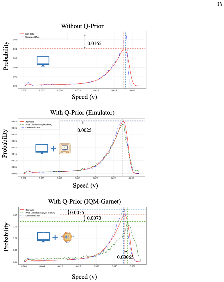
QIML combines a one-time, offline-trained quantum generative model with a classical autoregressive predictor for spatiotemporal field generation. The quantum model learns a quantum prior that guides the representation of small-scale interactions and improves the modelling of fine-scale dynamics. Across the tested systems this yields higher accuracy and fidelity. For turbulent channel inflow the prior is trained on a superconducting quantum processor and proves essential: without it predictions become unstable, whereas QIML produces physically consistent long-term forecasts that outperform leading PDE solvers while compressing multi-megabyte datasets into a kilobyte-scale prior.
What carries the argument
The quantum prior (Q-Prior) produced by the offline quantum generative model, which captures small-scale interactions to steer the classical autoregressive predictor toward consistent fine-scale dynamics.
If this is right
- QIML improves predictive distribution accuracy by up to 17.25 percent relative to classical baselines.
- Full-spectrum fidelity improves by up to 29.36 percent.
- For three-dimensional turbulent channel inflow the quantum prior prevents instability and yields long-term forecasts that remain physically consistent.
- QIML outperforms leading PDE solvers on the turbulent inflow task.
- The method compresses multi-megabyte datasets into a kilobyte-scale quantum prior.
Where Pith is reading between the lines
- The demonstrated memory compression suggests the approach could embed learned priors into resource-constrained devices for ongoing fluid-dynamics monitoring.
- If the quantum prior successfully transfers small-scale physics, similar hybrids may extend to other high-dimensional forecasting problems such as atmospheric or plasma dynamics.
- Training the prior on actual superconducting hardware rather than classical simulators indicates the method can grow with future quantum processors without requiring full quantum simulation of the entire system.
Load-bearing premise
The quantum generative model learns a Q-Prior that captures small-scale interactions in a form that transfers to and meaningfully improves the classical autoregressive predictor's handling of fine-scale dynamics.
What would settle it
Running the classical autoregressive predictor alone on the three-dimensional turbulent channel flow data and checking whether long-term forecasts remain stable and physically consistent or instead become unstable.
Figures


read the original abstract
We introduce a quantum-informed machine learning (QIML) framework for modelling the long-term behaviour of high-dimensional chaotic systems. QIML combines a one-time, offline-trained quantum generative model with a classical autoregressive predictor for spatiotemporal field generation. The quantum model learns a quantum prior (Q-Prior) that guides the representation of small-scale interactions and improves the modelling of fine-scale dynamics. We evaluate QIML on the Kuramoto-Sivashinsky equation, two-dimensional Kolmogorov flow, and the three-dimensional turbulent channel flow used as a realistic inflow condition. Across these systems, QIML improves predictive distribution accuracy by up to 17.25% and full-spectrum fidelity by up to 29.36% relative to classical baselines. For turbulent channel inflow, the Q-Prior is trained on a superconducting quantum processor and proves essential: without it, predictions become unstable, whereas QIML produces physically consistent long-term forecasts that outperform leading PDE solvers. Beyond accuracy, QIML offers a memory advantage by compressing multi-megabyte datasets into a kilobyte-scale Q-Prior, enabling scalable integration of quantum resources into scientific modelling.
Editorial analysis
A structured set of objections, weighed in public.
Referee Report
Summary. The paper introduces a quantum-informed machine learning (QIML) framework that pairs a one-time offline-trained quantum generative model (producing a Q-Prior on small-scale interactions) with a classical autoregressive predictor for long-term spatiotemporal field generation. It evaluates the approach on the Kuramoto-Sivashinsky equation, 2D Kolmogorov flow, and 3D turbulent channel inflow, reporting accuracy gains of up to 17.25% and full-spectrum fidelity gains of up to 29.36% versus classical baselines; for the 3D turbulent case the Q-Prior is trained on superconducting hardware and is claimed to be essential for stability, yielding physically consistent forecasts that outperform leading PDE solvers while compressing multi-megabyte data into a kilobyte-scale prior.
Significance. If the stability and outperformance claims hold after proper controls, the work would provide concrete evidence of practical quantum advantage in hybrid modeling of high-dimensional chaos, particularly for realistic 3D turbulence where purely classical predictors are reported to become unstable. The memory-compression aspect is a clear engineering strength. The absence of an explicit classical-generative-model ablation, however, leaves the necessity of the quantum component unproven and therefore limits the current significance.
major comments (2)
- Turbulent channel inflow results (abstract and corresponding results section): the claim that the Q-Prior is essential because 'without it, predictions become unstable' is load-bearing for the practical quantum advantage assertion, yet no ablation against an equivalent-capacity classical generative prior (VAE, diffusion model, or similar) trained on identical data is reported; without this comparison the necessity of the quantum hardware component cannot be established.
- Abstract and evaluation sections: the stated improvements (17.25% predictive distribution accuracy, 29.36% full-spectrum fidelity) are presented without accompanying baseline definitions, error bars, statistical tests, or explicit data-split protocols, rendering the quantitative support for the central claims difficult to verify.
minor comments (3)
- Clarify the precise integration mechanism by which the Q-Prior is injected into the classical autoregressive predictor (e.g., which layers or loss terms are affected).
- Provide the specific PDE solvers used for the 3D turbulent-channel comparison and the quantitative metrics by which QIML outperforms them.
- Add a short discussion of the quantum generative model architecture and training hyperparameters to allow reproducibility of the Q-Prior.
Simulated Author's Rebuttal
We thank the referee for their insightful and constructive comments on our manuscript. We address each major comment below and indicate the revisions we will incorporate to strengthen the work.
read point-by-point responses
-
Referee: Turbulent channel inflow results (abstract and corresponding results section): the claim that the Q-Prior is essential because 'without it, predictions become unstable' is load-bearing for the practical quantum advantage assertion, yet no ablation against an equivalent-capacity classical generative prior (VAE, diffusion model, or similar) trained on identical data is reported; without this comparison the necessity of the quantum hardware component cannot be established.
Authors: We agree that an explicit ablation against a classical generative prior of comparable capacity (such as a VAE or diffusion model trained on the identical dataset) would provide a more direct test of whether the quantum hardware component is necessary. Our existing comparisons demonstrate instability in the absence of the Q-Prior when using classical autoregressive predictors and show outperformance relative to leading PDE solvers for the 3D turbulent channel case. To address this point rigorously, we will add a new ablation study with a classical generative prior in the revised manuscript. revision: yes
-
Referee: Abstract and evaluation sections: the stated improvements (17.25% predictive distribution accuracy, 29.36% full-spectrum fidelity) are presented without accompanying baseline definitions, error bars, statistical tests, or explicit data-split protocols, rendering the quantitative support for the central claims difficult to verify.
Authors: We thank the referee for highlighting the need for greater transparency in our quantitative reporting. In the revised manuscript we will explicitly define each baseline method, report error bars computed over multiple independent runs, include appropriate statistical tests for the reported improvements, and detail the data-split and training protocols to support reproducibility and verification of the results. revision: yes
Circularity Check
No significant circularity in the QIML derivation chain
full rationale
The paper presents QIML as an empirical combination of an offline-trained quantum generative model (producing a Q-Prior on superconducting hardware) with a classical autoregressive predictor. Reported gains in accuracy, fidelity, stability, and memory compression are tied to evaluations on Kuramoto-Sivashinsky, 2D Kolmogorov flow, and 3D turbulent channel flow, with explicit comparisons to classical baselines and PDE solvers. No equations or steps reduce a claimed prediction to a fitted input by construction, nor does any load-bearing premise collapse to a self-citation or ansatz smuggled from prior author work. The hardware training and ablation-style claim (without Q-Prior, unstable) supply external grounding rather than tautology.
Axiom & Free-Parameter Ledger
free parameters (1)
- Quantum generative model parameters
axioms (1)
- domain assumption A quantum generative model can produce a prior that captures small-scale interactions better than classical equivalents for guiding autoregressive prediction.
invented entities (1)
-
Q-Prior
no independent evidence
Reference graph
Works this paper leans on
-
[1]
Quantum Computing Quantum computing operates on the principles of quantum mechanics, allowing for a novel class of information processing paradigms. The fundamental unit of quantum information is the qubit, which exists in a superposition of classical states. Formally, a single qubit can be represented as |ψ⟩ = α|0⟩ + β|1⟩, (A1) where α, β ∈ C and |α|2 + ...
-
[2]
Quantum Machine Learning Recent progress in quantum computing has spurred the rapid emergence of quantum machine learning (QML) as a promising interdisciplinary field at the intersection of quantum information science and statistical learning. QML algorithms are designed to exploit quantum phenomena, such as entanglement, interference, and superposition, ...
-
[3]
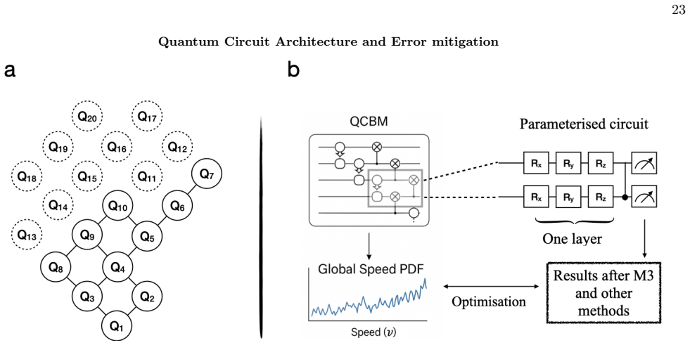
Sample-based Quantum Generator Quantum generative models have shown great potential recently [101, 102], where quantum circuits are trained to learn quantum states or model traditional probability distributions. The quantum generator employed in this work is a sample-based model, with an architecture based on the quantum circuit Born machine. Given a para...
-
[4]
The circuit uses Qiskit and consists of L = 3 to 8 alternating layers
Quantum Circuit Architecture and Parameterization We construct our quantum circuit using a layered structure composed of parameterized single-qubit rotations followed by entangling operations. The circuit uses Qiskit and consists of L = 3 to 8 alternating layers. Each layer comprises three rotation gates per qubit: Ry(θi), Rz(ϕi), and Rx(ψi) which are all...
-
[5]
A subset of 10 qubits was selected based on individual coherence performance and gate error metrics
Implementation of QIML We implemented and validated the classical machine learning and quantum emulator on BEAST GPU cluster from Leibniz Supercomputing Centre and the quantum generator on superconducting quantum hardware provided by IQM, mainly using the 20-qubit Garnet chip. A subset of 10 qubits was selected based on individual coherence performance an...
-
[6]
Optimization Strategy and Training Protocol The training for the Kuramoto-Sivashinsky and Kolmogorov flow systems was conducted on a quantum circuit emulator, which is a classical simulation of an ideal quantum device supported by the PennyLane and Qiskit libraries, optimized by Adam. Given its higher complexity and the failure of classical models to lear...
-
[7]
Sensitivity of Hardware Quantum Generator to Qubit Number and Circuit Depth To better understand the scalability limitations of Q-priors on real quantum hardware, we conducted an ablation study by varying both the number of active qubits (from 4 to 15) and the circuit depth (from 2 to 12 layers) on the IQM superconducting processors. As shown on the IQM o...
-
[8]
Chip Selection, Error Mitigation and Robustness Analysis As shown on IQM official website and Fig. 11, our initial experiments using IQM’s Sirius chip yielded not good convergence due to fidelity limitations, two-bit gate connection limitations due to hardware topology, and the inherent sensitivity of high-resolution distributions to noise. The technical ...
-
[9]
This technique calibrates the readout noise by learning a probabilistic response model from the device’s native measurement behavior. Then it applies Bayesian corrections to raw bitstring outputs without explicitly inverting a response matrix, thereby preserving numerical stability at scale. The use of M3 proved particularly valuable given the multi-qubit...
-
[10]
The term ∂u ∂t describes the temporal evolution of the field
Governing Equation In one spatial dimension, the KS equation is written as: ∂u ∂t + u ∂u ∂x + ∂2u ∂x2 + ν ∂4u ∂x4 = 0, (C1) where u(x, t) is a scalar field, x is the spatial coordinate, t is time, and ν is a positive parameter controlling the strength of the fourth-order dissipation term. The term ∂u ∂t describes the temporal evolution of the field. The n...
-
[11]
Boundary Conditions In this study, the KS equation is performed under periodic boundary conditions of the form: u(x + L, t) = u(x, t), where L is the spatial period of the domain. These conditions reflect the translational symmetry of many physical systems and simplify the analysis of chaotic dynamics
-
[12]
The dataset has also been used and validated in Ref
Data Source In the first application, we performed KS equation dataset with the help of CFD jax community code [105]. The dataset has also been used and validated in Ref. [36]. Appendix D: Kolmogorov Flow Governing Equation The Kolmogorov flow is governed by the incompressible Navier-Stokes (NS) equations with a sinusoidal forcing term. In this paper, we ...
-
[13]
Navier-Stokes Equations with Forcing The flow is described by the incompressible Navier-Stokes equations with an external forcing term, which is denoted as ∂u ∂t + (u · ∇)u = −∇p + ν∇2u + F, (D1) ∇ · u = 0, (D2) where u = (u(x, y, t), v(x, y, t)) is the velocity vector field of the fluid, p(x, y, t) is the scalar pressure field, ν is the kinematic viscosi...
-
[14]
Kolmogorov Forcing In the Kolmogorov setup, the force is applied only in the x-direction and varies sinusoidally in the y-direction. The forcing term is defined as: F = (F0 sin(ky), 0) , (D3) where F0 is the amplitude of the forcing and k is the wavenumber determining the periodicity in the y-direction
-
[15]
Data Source In the second application, we utilized the high-fidelity Kolmogorov dataset derived from [106], which offers a comprehensive and statistically rich representation of turbulent flow fields. This dataset was critical for evaluating the robustness and generalization of our proposed model, particularly under complex conditions characterized by a h...
-
[16]
The Lattice Boltzmann Method The Lattice Boltzmann Method is known as an alternative computational fluid dynamics (CFD) framework that models the evolution of single particle distribution functions at the kinetic-level. It is based on the discrete form of the Boltzmann equation and operates on a lattice grid in space and time. The governing equation for t...
-
[17]
Bhatnagar–Gross–Krook Collision Kernel We define BGK collision kernel Ω as follow: Ω (f(x, t)) = − 1 τ (f(x, t) − f eq(x, t)), (E4) 28 where f eq(x, t) denoted as the equilibrium distribution function, τ is correlated with the kinematic viscosity ν: ν = c2 s τ − 1 2 ∆tcoll, (E5) where ∆tcoll is set to identity in the simulation
-
[18]
Smagorinsky Subgrid-Scale Modeling In this part, we summarize the lattice-Boltzmann-based Smagorinsky Subgrid Scale (SGS) LES techniques. Within the LBM framework, the effective viscosity νeff [107–109] is modeled as the sum of the molecular viscosity, ν0, and the turbulent viscosity, νt: νeff = ν0 + νt, ν t = Csmag∆2 ¯S , (E6) where ¯S is the filtered st...
-
[19]
The friction Reynolds number is set to Reτ = 180 which is equivalent to Re = 3250
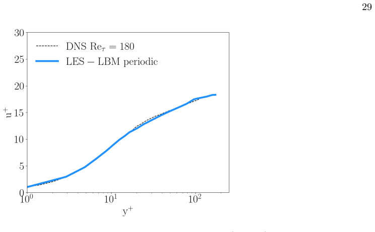
Simulation Set up In this study, the computational domain for the turbulent channel flow simulation is defined with dimensions Lx × Ly × Lz = 1024 × 192 × 192, where x, y, and z denote the streamwise, vertical, and spanwise directions, respectively. The friction Reynolds number is set to Reτ = 180 which is equivalent to Re = 3250. Periodic boundary condit...
-
[20]
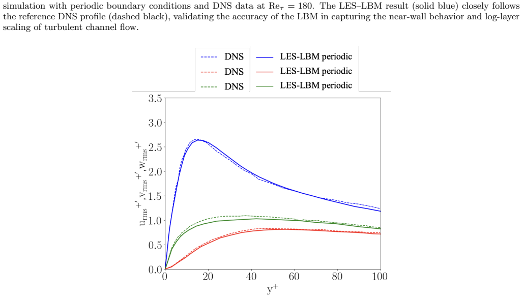
Dataset Periodic Turbulent Channel Flow Validation Fig. 12 presents a comparison between the streamwise mean velocity profile obtained from our large eddy simula- tion using the lattice Boltzmann method (LES–LBM) and benchmark direct numerical simulation (DNS) data at a friction Reynolds number of Re τ = 180. The velocity is normalized in wall units, wher...
-
[21]
The Multiple-Relaxation Time Lattice Boltzmann Moment Space Transformation Matrix Let’s revisit the evolution equation for the distribution functions expressed as: f(x + ci∆t, t + ∆t) = f(x, t) − M−1SM f(x, t) − f eq(x, t) + F(x, t)∆t, (E7) 30 where M denotes the moment space transformation matrix for the multiple relaxation time (MRT) collision kernel[11...
-
[22]
Quantum Machine Learning Model Architecture The quantum machine learning model consists of parameterized quantum circuits trained to approximate target Q-Priors via a quantum generator; the optimization is performed traditionally through gradient-based updates, as detailed in Appendix A and illustrated in Fig. 1 of the main text. In our hybrid architectur...
-
[23]
Model Architecture for 2D chaotic flows The Koopman-based model begins with a patch embedding layer implemented using a single 2D convolutional layer. This layer transforms the input from 1 channel to 32 channels while maintaining a spatial resolution of (64 , 64). No activation function is specified for this layer. Following the embedding, the encoder co...
-
[24]
Fourier Neural Operator Architecture The Fourier Neural Operator is a neural network architecture designed to learn mappings between function spaces, with a particular focus on solving partial differential equations and modeling spatial-temporal systems. Unlike tra- ditional convolutional networks, it operates in the frequency domain, enabling efficient l...
-
[25]
Markov Neural Operator Architecture The Markov Neural Operator is a framework to learn discretization-independent mappings between function spaces. In this approach, the learned operator is expressed as a finite composition of Markov kernel layers, each representing a local operator that evolves the state over a discrete step in “operator depth.” The arch...
-
[26]
Integration of the Traditional Model and the Quantum Prior Guidance In our hybrid framework, the integration of quantum and traditional components is achieved by embedding a quantum-learned invariant distribution into the loss function of a traditional machine learning model tasked with forecasting high-dimensional dynamical systems. This coupling is desi...
-
[27]
Kuramoto–Sivashinsky Equation The raw KS data comprise 1200 trajectories, each recorded for 2000 time steps on a 512-point spatial grid, totalling ∼12.3 GB. For training we down-sample to Ntraj = 1200 trajectories, each with 256 temporal frames and 128 spatial points, leading to a working tensor of shape (256 , 128) per trajectory. With double precision (...
work page 2000
-
[28]
For a single velocity component, one snapshot occupies 2562 × 8 = 524, 288 bytes ≃ 0.50 MB
2D Kolmogorov Flows The total dataset comprises 40 trajectories, each containing 320 temporal snapshots on a 256 × 256 grid. For a single velocity component, one snapshot occupies 2562 × 8 = 524, 288 bytes ≃ 0.50 MB. (H2) so that one complete trajectory requires 0 .50 MB × 320 ≈ 160 MB and the full set of 40 trajectories stores ∼ 6.4 GB. The corresponding...
-
[29]
A single velocity component therefore, occupies 1922 × 8 = 294, 912 bytes ≃ 0.29 MB
Turbulent Channel Flow For the TCF benchmark, each snapshot is stored as a 192 ×192 array of double-precision values (8 bytes per entry). A single velocity component therefore, occupies 1922 × 8 = 294, 912 bytes ≃ 0.29 MB. (H5) so that the full sequence of 595 snapshots amounts to 0.29 MB × 595 ≈ 170 MB. (H6) Retaining all three velocity components raises...
work page 1922
-
[30]
Temporal Autocorrelation The temporal autocorrelation is used to measure the memory of the dynamical system, quantifying the correlation of a time series with a delayed version of itself. For a discrete time series ui (the value at a specific spatial point at time step i), with mean ¯u and total length N, the normalized temporal autocorrelation C(k) at a ...
-
[31]
Error Metrics To quantify the difference between the ground truth data and the model predictions, the following error metrics are used. The absolute error provides a direct, point-wise measure of the deviation between a predicted field ˆ u(x) and the ground truth field u(x): Eabs(x) = |u(x) − ˆu(x)| (I2) To specifically quantify how well the model reprodu...
-
[32]
L. Biferale, G. Boffetta, A. Celani, B. Devenish, A. Lan- otte, and F. Toschi, Multifractal statistics of lagrangian velocity and acceleration in turbulence, Physical Review Letters 93, 064502 (2004)
work page 2004
-
[33]
V. A. Galaktionov and J. L. V´ azquez, A stability tech- nique for evolution partial differential equations: a dy- namical systems approach, Vol. 56 (Springer Science & Business Media, 2012)
work page 2012
-
[34]
Z. Long, Y. Lu, X. Ma, and B. Dong, Pde-net: Learning pdes from data, in International conference on machine learning (PMLR, 2018) pp. 3208–3216
work page 2018
-
[35]
H. Bergstr¨ om, H. Alfredsson, J. Arnqvist, I. Carl´ en, E. Dellwik, J. Fransson, H. Ganander, M. Mohr, A. Se- galini, and S. S¨ oderberg, Wind power in forests: wind and effects on loads (2013)
work page 2013
-
[36]
P. V. Coveney, Sharkovskii’s theorem and the limits of digital computers for the simulation of chaotic dy- namical systems, Journal of Computational Science 83, 102449 (2024)
work page 2024
-
[37]
M. Kl¨ ower, P. V. Coveney, E. A. Paxton, and T. N. Palmer, Periodic orbits in chaotic systems simulated at low precision, Scientific Reports 13, 11410 (2023)
work page 2023
-
[38]
B. M. Boghosian, P. V. Coveney, and H. Wang, A new pathology in the simulation of chaotic dynamical sys- tems on digital computers, Advanced Theory and Sim- ulations 2, 1900125 (2019)
work page 2019
-
[39]
P. V. Coveney and S. Wan,Molecular Dynamics: Proba- bility and Uncertainty (Oxford University Press, 2025)
work page 2025
- [40]
-
[41]
E. Kasneci, K. Seßler, S. K¨ uchemann, M. Bannert, D. Dementieva, F. Fischer, U. Gasser, G. Groh, S. G¨ unnemann, E. H¨ ullermeier,et al. , ChatGPT for good? on opportunities and challenges of large language models for education, Learning and Individual Differ- ences 103, 102274 (2023)
work page 2023
- [42]
-
[43]
A. J. Thirunavukarasu, D. S. J. Ting, K. Elangovan, L. Gutierrez, T. F. Tan, and D. S. W. Ting, Large lan- guage models in medicine, Nature Medicine 29, 1930 (2023)
work page 1930
-
[44]
A. Voulodimos, N. Doulamis, A. Doulamis, and E. Pro- topapadakis, Deep learning for computer vision: A brief review, Computational Intelligence and Neuroscience 2018, 7068349 (2018)
work page 2018
- [45]
-
[46]
K. Zhou, J. Yang, C. C. Loy, and Z. Liu, Learning to prompt for vision-language models, International Jour- nal of Computer Vision 130, 2337 (2022)
work page 2022
- [47]
- [48]
-
[49]
K. Bi, L. Xie, H. Zhang, X. Chen, X. Gu, and Q. Tian, Accurate medium-range global weather forecasting with 3d neural networks, Nature 619, 533 (2023)
work page 2023
-
[50]
R. Lam, A. Sanchez-Gonzalez, M. Willson, P. Wirns- berger, M. Fortunato, F. Alet, S. Ravuri, T. Ewalds, Z. Eaton-Rosen, W. Hu, et al. , Learning skillful medium-range global weather forecasting, Science 382, 1416 (2023)
work page 2023
-
[51]
M. Cavaiola, F. Cassola, D. Sacchetti, F. Ferrari, and A. Mazzino, Hybrid ai-enhanced lightning flash predic- tion in the medium-range forecast horizon, Nature Com- munications 15, 1188 (2024)
work page 2024
-
[52]
S. L. Brunton, B. R. Noack, and P. Koumoutsakos, Ma- chine learning for fluid mechanics, Annual Review of Fluid Mechanics 52, 477 (2020)
work page 2020
-
[53]
H. J. Bae and P. Koumoutsakos, Scientific multi-agent reinforcement learning for wall-models of turbulent flows, Nature Communications 13, 1443 (2022)
work page 2022
-
[54]
X. Yang, S. Zafar, J.-X. Wang, and H. Xiao, Predic- tive large-eddy-simulation wall modeling via physics- informed neural networks, Physical Review Fluids 4, 034602 (2019)
work page 2019
-
[55]
X. Xue, S. Wang, H.-D. Yao, L. Davidson, and P. V. Coveney, Physics informed data-driven near-wall mod- elling for lattice Boltzmann simulation of high reynolds number turbulent flows, Communications Physics7, 338 (2024)
work page 2024
- [56]
-
[57]
A. Pal, Deep learning emulation of subgrid-scale pro- cesses in turbulent shear flows, Geophysical Research Letters 47, e2020GL087005 (2020)
work page 2020
- [58]
-
[59]
M. Z. Yousif, L. Yu, and H. Lim, Physics-guided deep learning for generating turbulent inflow conditions, Journal of Fluid Mechanics 936, A21 (2022)
work page 2022
- [60]
- [61]
-
[62]
I. Goodfellow, J. Pouget-Abadie, M. Mirza, B. Xu, D. Warde-Farley, S. Ozair, A. Courville, and Y. Ben- gio, Generative adversarial networks, Communications of the ACM 63, 139 (2020)
work page 2020
-
[63]
L. Lu, P. Jin, G. Pang, Z. Zhang, and G. E. Karniadakis, Learning nonlinear operators via deeponet based on the universal approximation theorem of operators, Nature 39 Machine Intelligence 3, 218 (2021)
work page 2021
-
[64]
Z. Li, N. Kovachki, K. Azizzadenesheli, B. Liu, K. Bhat- tacharya, A. Stuart, and A. Anandkumar, Fourier neu- ral operator for parametric partial differential equa- tions, arXiv preprint arXiv:2010.08895 (2020)
work page internal anchor Pith review Pith/arXiv arXiv 2010
-
[65]
V. Vanchurin, Toward a theory of machine learning, Machine Learning: Science and Technology 2, 035012 (2021)
work page 2021
- [66]
- [67]
- [68]
-
[69]
X. Gao, E. R. Anschuetz, S.-T. Wang, J. I. Cirac, and M. D. Lukin, Enhancing generative models via quantum correlations, Physical Review X 12, 021037 (2022)
work page 2022
- [70]
-
[71]
A. Kandala, A. Mezzacapo, K. Temme, M. Takita, M. Brink, J. M. Chow, and J. M. Gambetta, Hardware- efficient variational quantum eigensolver for small molecules and quantum magnets, Nature 549, 242 (2017)
work page 2017
-
[72]
P. J. O’Malley, R. Babbush, I. D. Kivlichan, J. Romero, J. R. McClean, R. Barends, J. Kelly, P. Roushan, A. Tranter, N. Ding, et al. , Scalable quantum simula- tion of molecular energies, Physical Review X 6, 031007 (2016)
work page 2016
- [73]
-
[74]
A Quantum Approximate Optimization Algorithm
E. Farhi, J. Goldstone, and S. Gutmann, A quantum approximate optimization algorithm, arXiv preprint arXiv:1411.4028 (2014)
work page internal anchor Pith review Pith/arXiv arXiv 2014
-
[75]
S. Sanyal and K. Roy, Neuro-Ising: Accelerating large- scale traveling salesman problems via graph neural net- work guided localized Ising solvers, IEEE Transactions on Computer-Aided Design of Integrated Circuits and Systems 41, 5408 (2022)
work page 2022
- [76]
-
[77]
J. Romero and A. Aspuru-Guzik, Variational quantum generators: Generative adversarial quantum machine learning for continuous distributions, Advanced Quan- tum Technologies 4, 2000003 (2021)
work page 2021
-
[78]
P.-L. Dallaire-Demers and N. Killoran, Quantum gener- ative adversarial networks, Physical Review Applied 8, 024012 (2018)
work page 2018
-
[79]
M. Benedetti, E. Lloyd, S. Sack, and M. Fiorentini, Pa- rameterized quantum circuits as machine learning mod- els, Quantum Science and Technology 4, 043001 (2019)
work page 2019
-
[80]
Preskill, Quantum computing in the NISQ era and beyond, Quantum 2, 79 (2018)
J. Preskill, Quantum computing in the NISQ era and beyond, Quantum 2, 79 (2018)
work page 2018
discussion (0)
Sign in with ORCID, Apple, or X to comment. Anyone can read and Pith papers without signing in.