REVIEW 4 major objections 5 minor 8 references
Deep Uzawa for Kinetic Transport with Lagrange-Enforced Boundaries
T0 review · 4 major / 5 minor · reviewed 2026-08-06 · deepseek-v4-flash
Pith's one-line read Deep Uzawa trains a neural network against a Lagrange multiplier so that inflow boundary data are enforced exactly in the limit, not merely penalised.
desk verdict The continuum Uzawa analysis is solid and the transport setting is a real addition, but the neural convergence theorem leans on an unstated convexity assumption and the experiments don't yet verify the main claim. read the letter →
The pith
A machine-rendered reading of the paper's core claim, the machinery that carries it, and where it could break.
The reading
What carries the argument
The object that carries the argument is the saddle-point Lagrangian $L(u,\lambda)=J(u)-\langle\lambda,u-g\rangle_{L^2(\Gamma^-)}$, where $J(u)=\frac12\|(T+S)u\|^2_{L^2(W)}+\frac\gamma2\|u-g\|^2_{L^2(\Gamma^-)}$, paired with the Uzawa updates $u_k=\arg\min_{u\in V}L(u,\lambda_k)$ and $\lambda_{k+1}=\lambda_k+\rho(u_k-g)$ on the inflow boundary. The proof runs through two identities: the residual identity, which equates the primal error in the graph norm with the dual pairing $\langle\lambda_k-\lambda^*,u_k-u^*\rangle$, and the multiplier distance recursion, whose combination yields a telescoping sum that forces both $\|(T+S)(u_k-u^*)\|_{L^2(W)}$ and $\|u_k-u^*\|_{L^2(\Gamma^-)}$ to zero when $0<\rho<2\gamma$. For the discrete neural version, Theorem 5.1 and Lemma 5.4 control the inner minimisation error by assuming the discretised Lagrangian is strongly convex with Lipschitz gradient in parameter space, and Lemma 5.2 supplies network density in the $V$-norm.
What would settle it
Run Algorithm 1 on Example 1 while recording the inner suboptimality gap $\delta_k$ at each outer iteration and the expected boundary residual $\mathbb{E}\|u_k^\theta-g\|^2_{L^2(\Gamma^-)}$; if $\delta_k$ plateaus above zero as inner gradient steps grow, or if the boundary residual stops decreasing at a positive level, the convergence-in-expectation theorem is not borne out in that setting.
Extended reading notes
Core claim
The central claim, formalised in Theorem 5.7 and Corollary 5.8, is that the neural Uzawa iterates converge in expectation to the exact solution in the $V$-norm, and that the expected boundary residual in $L^2(\Gamma^-)$ tends to zero. At the continuum level, Theorem 3.5 shows the exact Uzawa iterates converge in the graph norm of the transport operator whenever the step size satisfies $0<\rho<2\gamma$, and Theorem 3.7 strengthens this to a norm that also controls the spatial derivative and both boundary traces when absorption dominates scattering. The paper positions this as the key contrast with penalty-based neural solvers, where boundary errors typically persist in the limit.
Load-bearing premise
The proof depends on two unproved properties for the multilayer networks it trains: that each inner optimisation over parameters is convex enough for the claimed gradient-descent rate, and that the multiplier sequence converges to the exact multiplier.
Editorial extensions
If this is right
- The continuum Uzawa iteration converges in the graph norm of the transport operator whenever the step size satisfies $0<\rho<2\gamma$.
- If absorption dominates scattering, the iterates converge in a stronger norm that also controls the spatial derivative and both boundary traces.
- Under smoothness, network density in $V$, Monte Carlo quadrature consistency, and summable inner-minimisation errors, the neural iterates converge in expectation to the exact solution in the $V$-norm.
- The expected inflow boundary residual $\mathbb{E}\|u_k^\theta-g\|^2_{L^2(\Gamma^-)}$ tends to zero, so the boundary condition is enforced asymptotically rather than only through a penalty.
- The method handles scattering and heterogeneous absorption because the transport operator and scattering kernel enter the Lagrangian directly, and the experiments demonstrate anisotropic transport, shadowing, and forward-peaked scattering.
Reading between the lines
- The authors leave implicit that the same saddle-point construction could be applied to time-dependent transport or to inverse problems; the paper establishes only the stationary forward problem, so those would be genuine extensions rather than corollaries.
- A testable extension is to replace the fully connected network with a parameterisation that is convex in the parameters, such as a linear or kernel ansatz; under that choice the convexity premise of Lemma 5.4 would hold by construction and the convergence theorem would apply rigorously.
- The asymptotic boundary enforcement suggests that the practical advantage over soft-penalty training should be measured on the boundary residual at matched computational cost; the paper's experiments show boundary loss decay but do not include that head-to-head comparison.
Editorial analysis
A structured set of objections, weighed in public.
Referee Report
Summary. The manuscript proposes Deep Uzawa, a mesh-free neural-network method for stationary linear transport equations with inflow boundary conditions. It introduces a saddle-point formulation in which a Lagrange multiplier on the inflow boundary enforces the trace condition, and it iterates an Uzawa scheme that alternates an inner primal minimization over the transport residual with a dual update of the boundary multiplier. The paper proves convergence of the continuum Uzawa iteration (Section 3), analyzes the neural/discrete scheme through a decomposition into approximation, quadrature, and optimization errors (Section 5), and reports qualitative numerical experiments for directional transport, shadowing, scattering, noisy boundary data, and heterogeneous media (Section 6). The central claim, stated in Theorem 5.7 and Corollary 5.8, is that the neural iterates converge in expectation in the V-norm and that the inflow boundary residual vanishes asymptotically, in contrast to penalty-based PINNs.
Significance. The continuum part of the paper is a genuine contribution: the Uzawa formulation for transport is natural, and Theorem 3.5 gives a clean residual-identity proof of convergence that does not rely on coercivity. The paper also deserves credit for attempting a full error decomposition and for being explicit that the convergence statements are in expectation. However, the headline neural convergence claim is not currently established: Lemma 5.4 applies convex optimization rates to a nonconvex parameter objective, Theorem 5.7 invokes dual convergence that is neither proved nor assumed in the theorem statement, and Section 6 provides no quantitative validation. If these gaps are addressed, the method would be of interest to the scientific-machine-learning community, but in its present form the manuscript overclaims relative to what is proved.
major comments (4)
- [Section 5.4, Eqs. (77)-(81)] Lemma 5.4 applies Nesterov's convex-rate bound to F(θ)=L_h(u_θ, λ~_k; ξ_k). For the tanh/GELU/SiLU feedforward networks of Section 4.1, the map θ ↦ u_θ is nonlinear, so F is not convex in θ; convexity of L_h in u does not transfer to parameter space. Consequently Eq. (80) and the bound δ_k ≤ C/T_k in Eq. (81) are not supported, and premise (93) of Theorem 5.7 lacks a mechanism. The authors should either restrict to parameter-convex architectures, e.g., input convex neural networks, or replace Lemma 5.4 with a convergence statement for nonconvex optimization whose assumptions are actually verified. The global L-Lipschitz gradient condition (78) and the uniform boundedness of θ_{k,0}−θ* used in Eq. (84) also need justification.
- [Section 5.7, Eq. (99), and Section 5.5, Eq. (85)] In the proof of Theorem 5.7, the convergence of the exact primal minimizers u_k to u* is justified by 'λ~_k → λ*' and continuity of the minimizer map. That dual convergence is not established anywhere: Theorem 3.5 yields summability of squared residuals and boundary errors, not convergence of λ_k to λ*, and Lemma 5.5 assumes λ~_k → λ† as a hypothesis. The argument is therefore circular at a load-bearing point. The authors should prove dual convergence, or state it as an explicit assumption in Theorem 5.7, and they should verify the continuity and coercivity assertions in Remark 5.6 rather than invoking them as standard facts.
- [Section 6, Examples 1-5] The experiments report only qualitative plots, loss histories, and visual statements such as 'captures directionality' and 'resolves scattering dynamics accurately.' There is no reference solution, no error metric, no mesh or grid baseline, and no comparison with a penalty-based PINN. To support the boundary-condition claim of Corollary 5.8, the paper should include quantitative boundary residuals and V-norm errors against a manufactured or highly accurate reference solution, with hyperparameters reported (network depth and width, NSGD, NUz, ρ, γ, and quadrature sizes). Without this, Section 6 cannot validate the method or the claimed convergence behavior.
- [Section 4.4 and Section 5.1/5.3] Algorithm 1 performs a fixed number NSGD of gradient steps and uses the quadrature formula (55), while Lemma 5.1 and Theorem 5.7 assume an inexact minimizer satisfying a suboptimality bound (57) and a Monte Carlo estimator L_h with i.i.d. samples and controllable bias (58), (98). The paper does not explain how the fixed-step implementation supplies the summable suboptimality errors ε_k and quadrature-consistency errors η_k, nor how the quadrature points of Eq. (55) are drawn from the uniform and inflow-weighted distributions used in Lemma 5.3. Without this link, the analysis is conditional on assumptions that Algorithm 1 may not satisfy.
minor comments (5)
- [Section 4.1, Eq. (50)] The statement that Θ := {θ ∈ R^P : u_θ ∈ V_N} is a linear subspace of R^P is confusing, since for a fixed architecture V_N is exactly the set of all parameterized networks and Θ is simply R^P; the useful distinction is that u_θ is nonlinear in θ, not that the parameter set is a linear subspace.
- [Theorem 5.7 and Example 4] Theorem 5.7 assumes all functions are smooth, but Example 4 uses discontinuous and noisy inflow data; the paper should state whether that experiment is outside the theory or should add assumptions covering discontinuous boundary data.
- [Lemma 5.5] The notation is inconsistent: Lemma 5.5 assumes λ~_k → λ†, while Theorem 5.7 invokes λ~_k → λ*, and the proof of Lemma 5.5 identifies u(λ†) with u* without proving λ† = λ*. The relation between the two limit multipliers should be clarified.
- [Section 6] The experimental section does not report the network architecture, learning rate schedule, number of Uzawa and SGD steps, or quadrature sample sizes; these details are necessary for reproducibility and for interpreting the loss histories in Figures 1-5.
- [General] There are minor typographical and presentation issues, including the duplicated residual identity displayed in Eqs. (17) and (20) and the inconsistent use of λ† and λ* described above.
Circularity Check
No construction-level circularity: the continuum analysis is self-contained and the neural theorem is conditional rather than self-referential; the proof gaps are missing justifications, not circular reductions.
full rationale
The paper's derivation chain contains no step in which a claimed prediction is identical to a fitted input or in which a load-bearing result is justified only by the authors' prior work. The continuum Uzawa convergence (Theorems 3.5 and 3.7) is proved from the residual identity (17) and multiplier recursion (21), both algebraic consequences of the saddle-point optimality conditions; the conclusion follows from a telescoping-sum argument, not from a restatement of the V-norm definition. The neural convergence claim (Theorem 5.7) is explicitly conditional on the suboptimality bound (93), which is a stated hypothesis rather than a consequence of the desired convergence. The proof's invocation 'Since λ~_k → λ∗' near equation (99) is an unproved premise and Lemma 5.4 applies Nesterov's convex-rate bound to a map that is not proved convex for the stated tanh/GELU/SiLU networks; these are correctness and completeness gaps, not circular reductions. Self-citations [MPP24a] and [MPP24b] appear only in contextual or motivational remarks, and the supporting analysis is either re-derived in the paper or cited to independent references ([Nes13], [SZ19], [Yar18], [Dah+12]). The numerical boundary-enforcement reports are evaluations of a fitting objective, not independent predictions. Overall, no circularity under the strict definition used here.
Assumptions & free parameters
free parameters (5)
- penalty weight gamma
- Uzawa step size rho
- training hyperparameters (learning rate eta, SGD steps NSGD, Uzawa steps NUz, network width and depth)
- quadrature sample sizes N and M
- strong convexity constant mu and Lipschitz constant L
assumptions (5)
- domain assumption A saddle point (u*, lambda*) of the Lagrangian (14) exists and is unique.
- ad hoc to paper The map theta -> Lh(u_theta, lambda, xi) is convex and L-smooth in the network parameters.
- ad hoc to paper The dual iterates lambda_k converge to lambda* or lambda_dagger.
- domain assumption Neural networks with smooth activations are dense in the transport graph space V.
- domain assumption Monte Carlo integrands are uniformly bounded and Lipschitz for all iterates.
Cite this review
Pith. "Pith review of Deep Uzawa for Kinetic Transport with Lagrange-Enforced Boundaries." pith.science (2026). https://pith.science/paper/ZA7XRRER
@misc{pith2026250719907,
  author       = {Pith},
  title        = {Pith review of: Deep Uzawa for Kinetic Transport with Lagrange-Enforced Boundaries},
  year         = {2026},
  howpublished = {\url{https://pith.science/paper/ZA7XRRER}},
  note         = {Machine review of arXiv:2507.19907}
}
read the original abstract
We propose a neural network framework for solving stationary linear transport equations with inflow boundary conditions. The method represents the solution using a neural network and imposes the boundary condition via a Lagrange multiplier, based on a saddle-point formulation inspired by the classical Uzawa algorithm. The scheme is mesh-free, compatible with automatic differentiation and extends naturally to problems with scattering and heterogeneous media. We establish convergence of the continuum formulation and analyse the effects of quadrature error, neural approximation and inexact optimisation in the discrete implementation. Numerical experiments show that the method captures anisotropic transport, enforces boundary conditions and resolves scattering dynamics accurately.
Figures
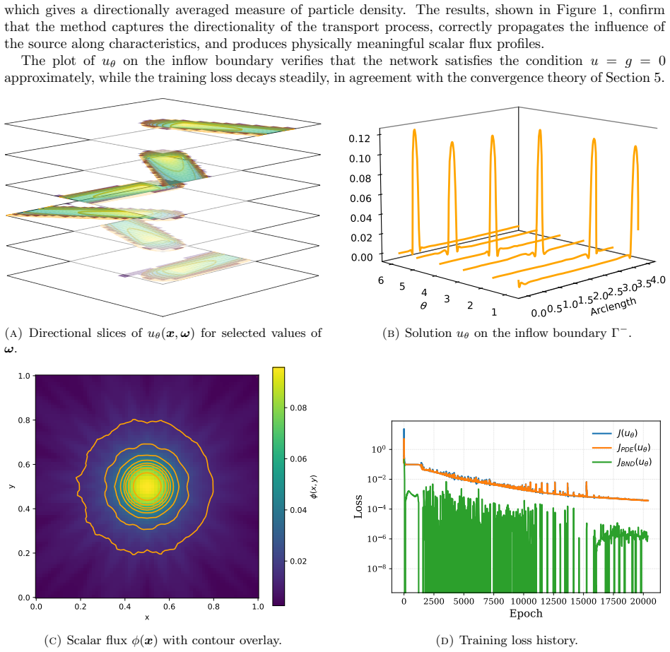


Figures from the paper (2 more)


Reference graph
Works this paper leans on
-
[1]
[AK17a] B. Amos and J. Z. Kolter. “Input convex neural networks”. In: Proceedings of the 34th Interna- tional Conference on Machine Learning . 2017, pp. 146–155. [AK17b] B. Amos and J. Z. Kolter. “Optnet: Differentiable optimization as a layer in neural networks”. In: International conference on machine learning . PMLR. 2017, pp. 136–145. [Ash+25] B. S. A...
work page 2025
-
[5]
Numerical solution of saddle point problems
Diagnostics for a heterogeneous medium. The solution exhibits appropriate attenuation across the absorption interface without oscil- lations, and the training process remains stable. [BGL05] M. Benzi, G. H. Golub, and J. Liesen. “Numerical solution of saddle point problems”. In: Acta numerica 14 (2005), pp. 1–137. [Bir94] G. A. Bird. Molecular gas dynamic...
work page 2005
-
[52]
Adaptive activation functions acceler- ate convergence in deep and physics-informed neural networks
[JKK20] A. D. Jagtap, K. Kawaguchi, and G. E. Karniadakis. “Adaptive activation functions acceler- ate convergence in deep and physics-informed neural networks”. In: Journal of Computational Physics 404 (2020), p. 109136. [KF24] J. Kotary and F. Fioretto. “Learning constrained optimization with deep augmented lagrangian methods”. In: arXiv preprint arXiv:...
arXiv 2020
-
[1994]
[BS23] S. Basir and I. Senocak. “An adaptive augmented lagrangian method for training physics and equality constrained artificial neural networks”. In: arXiv preprint arXiv:2306.04904 (2023). [Cal+25] A. Calloo et al. “Cycle-free polytopal mesh sweeping for Boltzmann transport”. In: Numerical Algorithms (2025), pp. 1–24. [Cer88] C. Cercignani. “The boltzm...
arXiv 2023
-
[2004]
A mixed variational framework for the radiative transfer equa- tion
[ES12] H. Egger and M. Schlottbom. “A mixed variational framework for the radiative transfer equa- tion”. In: Mathematical Models and Methods in Applied Sciences 22.03 (2012), p. 1150014. [Hin+08] M. Hinze et al. Optimization with PDE constraints. Vol
work page 2012
-
[2005]
[RPK19] M. Raissi, P. Perdikaris, and G. E. Karniadakis. “Physics-informed neural networks: A deep learning framework for solving forward and inverse problems involving nonlinear partial differ- ential equations”. In: Journal of Computational Physics 378 (2019), pp. 686–707. [SCH23] H. Son, S. W. Cho, and H. J. Hwang. “Enhanced physics-informed neural net...
work page 2019
-
[2008]
Solving high-dimensional partial differential equations using deep learning
[HJE18] J. Han, A. Jentzen, and W. E. “Solving high-dimensional partial differential equations using deep learning”. In: Proceedings of the National Academy of Sciences 115.34 (2018), pp. 8505–
work page 2018
-
[8510]
[Hou+24] P. Houston et al. “Efficient high-order space-angle-energy polytopic discontinuous Galerkin finite element methods for linear Boltzmann transport”. In: Journal of Scientific Computing 100.2 (2024), p
work page 2024
Reviewed August 6, 2026 · model on record in the stance chip above.
Discussion (0). Sign in to comment.