REVIEW 3 major objections 3 minor 81 references
Thermal Behavior of Generalized Black-Bounce Black Hole Model
T0 review · 3 major / 3 minor · reviewed 2026-08-15 · deepseek-v4-flash
Pith's one-line read Generalized black-bounce black holes get colder as the bounce parameter and deformation index grow, producing regular spacetimes with suppressed Hawking radiation.
desk verdict The stress-test is right: the paper's Hawking-temperature plots are internally inconsistent with its own metrics, so the central thermal claim does not stand. read the letter →
The pith
A machine-rendered reading of the paper's core claim, the machinery that carries it, and where it could break.
The reading
What carries the argument
The load-bearing object is the generalized black-bounce line element $ds^2=f(r)dt^2-f(r)^{-1}dr^2-\Sigma^2(r)(d\theta^2+\sin^2\theta\,d\phi^2)$ in Buchdahl form, with $\Sigma(r)=\sqrt{r^2+a^2}$ and $f(r)=1-2M(r)/\Sigma(r)$, where $M(r)$ is one of several mass functions designed to smooth the central region. The Hernandez–Misner–Sharp quasi-local mass, $M_{\rm HMS}(r)=\frac12\Sigma(r)[1-f(r)\Sigma'(r)^2]$, supplies the regularity and positivity checks, and the Hamilton–Jacobi tunneling derivation of the Hawking temperature, $T_{\rm BH}=A'(r_H)/(4\pi)$, converts the near-horizon slope of the metric function into a thermal statement. The argument works by combining these two tools: the mass function shapes $f(r)$ and its roots, and the slope at a horizon sets the temperature.
What would settle it
Pick the $n=1,k=2$ model, list all roots of $f(r)=0$, and compute $f'(r_H)$ at the outermost horizon; if the temperature no longer decreases monotonically with $a$ or vanishes at different parameter values, the central thermal claim fails. Separately, write down the total matter action whose field equations reproduce the stress-energy tensor from Section 2 for that model; if no causal energy-momentum source exists, the physical-admissibility claim is unsupported.
Extended reading notes
Core claim
The central claim is that the geometry $$f(r)=1-\frac{2M(r)}{\Sigma(r)},\quad \Sigma(r)=\sqrt{$r^{2}$+$a^{2}$},$$ with mass profiles $M(r)$ given in Eqs. (20), (28), (34), and (38), defines nonsingular black-bounce black holes whose Hawking temperature is $T_{\rm BH}=f'(r_H)/(4\pi)$ and falls when the bounce parameter $a$ or the deformation index $n$ increases. Each model tends to Schwarzschild as $a\to0$ and, for suitable parameters, to the Simpson–Visser spacetime as a base case. The paper further claims all models satisfy the regularity criteria of finite curvature invariants and smooth metric functions, and have positive quasi-local mass $M_{\rm HMS}(r)$ that runs from $a/2$ at the core to $m$ at infinity. On the thermal side, the temperature curves show characteristic peaks and zeros in the $(a,m)$ plane, so the models are taken to interpolate between radiative and effectively non-radiative, extremal-like states.
Load-bearing premise
The paper assumes the proposed metrics are physically realizable regular black holes, yet it never constructs the matter Lagrangian or field configuration whose anisotropic stress-energy tensor would generate them; it also leaves unspecified which horizon root is used when evaluating $T_{\rm BH}=f'(r_H)/(4\pi)$ for solutions with multiple horizons.
Editorial extensions
If this is right
- Larger bounce parameter $a$ generally lowers the Hawking temperature, so these regular geometries radiate less intensely than Schwarzschild black holes of the same mass.
- Zero-temperature points in parameter space act like extremal configurations where radiation switches off, offering candidate stable remnants at the end of evaporation.
- Because $a\to0$ recovers Schwarzschild and $n\to0$ recovers Simpson–Visser in several models, the family provides a continuous interpolation between classical and regular thermodynamics.
- The typically negative energy density outside the outer horizon means any realistic embedding needs exotic matter or a modified-gravity source, which the paper identifies but does not construct.
- The temperature peaks in the $(a,m)$ and $(n,m)$ planes locate transitions between radiative and suppressed phases, giving concrete predictions that future numerical or observational studies could test.
Reading between the lines
- Because the tunneling formula is evaluated at a horizon root without specifying which root is chosen, the claimed monotonic suppression with $a$ could change if the outermost horizon is selected instead of an inner one; a systematic root-selection rule would settle this.
- The same construction may extend to rotating or asymptotically de Sitter versions of these mass profiles, since the regularity checks are local; such extensions are not in the paper but follow naturally from its method.
- If the zero-temperature states are real, they suggest an observable signature: a population of compact remnants with no Hawking flux, which might be distinguished from ordinary black holes by the absence of thermal emission.
- A direct matter action reproducing the anisotropic stress–energy tensor would make the energy-condition violations concrete and is the most needed next step; the paper only works at the metric level.
Signed reviews
Editorial analysis
A structured set of objections, weighed in public.
Referee Report
Summary. The manuscript proposes a family of static, spherically symmetric 'generalized black-bounce' spacetimes with areal radius Σ(r)=√(r²+a²) and several choices of mass function M(r): a power-law family in Eq. (20), a cosine model in Eq. (28), an arctangent-product model in Eq. (34), and a pure arctangent model in Eq. (38). For each model the paper computes the Hernandez–Misner–Sharp quasi-local mass, discusses horizon structure and energy conditions, and derives the Hawking temperature through the Hamilton–Jacobi tunneling method, obtaining T=f'(r_H)/(4π). The central claims are that all geometries are regular, have positive and well-defined quasi-local masses, and that increasing the bounce parameter a or the deformation index n suppresses the Hawking temperature, implying reduced radiation and enhanced thermodynamic stability.
Significance. The construction is transparent and explicit: the metric functions are given in closed form, the HMS masses follow by direct substitution from Eq. (17), and the limiting behaviors such as M_HMS(0)=a/2 and M_HMS(∞)=m are easy to verify. The tunneling derivation, despite a sign typo in Eq. (46), leads to the standard surface-gravity temperature, and the regularity claim is supported by the smoothness of f and Σ with Σ>0. However, the quantitative thermal results as plotted are internally inconsistent with the stated metric functions: several reported temperatures occur for parameter values where no real horizon exists, and no horizon-selection rule is given for multi-horizon cases. These issues bear directly on the paper's central claim, so the present version cannot be accepted as is.
major comments (3)
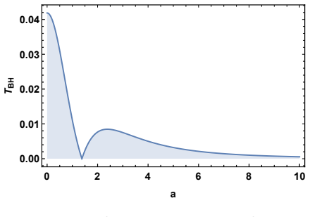
- [Section 4, Eq. (53), Figs. 14, 20, 22] The reported temperature curves are not consistent with the stated metrics because T=f'(r_H)/(4π) is evaluated without restricting to parameter values for which f(r) has a real root. For Model 3.4, Eq. (35) with n=m=1 gives f(r)=1-(4/(π r)) arctan(r/a); since arctan(r/a)/r is strictly decreasing, f increases from 1-4/(π a) to 1, so a horizon exists only for a<4/π≈1.273, whereas Fig. 20(a) reports a second temperature maximum at a≈3.6 where f(r)>0 everywhere. Similarly, Model 3.5, Eq. (39), has horizons only for a≲0.714 when n=m=1, yet Fig. 22(a) shows a second maximum at a≈4.2; and Model 3.1, Eq. (22), has horizons only for a<4/(3√3)≈0.770 when m=1, yet Fig. 14 reports a temperature zero at a≈1.45 and a second peak at a≈2.3. These are internal contradictions, not interpretive choices, and they invalidate the temperature-versus-parameter plots as presented.
- [Section 3, Eqs. (22), (29), and Section 4] For parameter values where the spacetime genuinely has two horizons (for example, Eq. (22) with m=1 and a=0.6), the paper does not state whether T is evaluated at the outer horizon, the inner horizon, or the degenerate extremal configuration. The surface gravity, and hence the temperature, differs between these horizons, and the monotonicity of T(a) can depend on the choice. Because the central claim about suppression of temperature with increasing a is extracted from these curves, the missing selection rule makes the central quantitative claim ambiguous even on the horizon branch.
- [Section 4, Figs. 12-23] The temperature plots are not reproducible from the text: no horizon-finding algorithm, no branch-selection rule, and no numerical data or code are provided. Given that the figures contain features that cannot arise from real roots of the stated f(r), the authors should specify exactly which equation was solved to produce each curve, and should regenerate all thermal plots using only genuine horizons.
minor comments (3)
- [Section 4, Eq. (46)] The leading-order WKB equation has the sign of the mass term wrong: from Eq. (44) one obtains (∂_tT)^2 - A^2(∂_rT)^2 + m^2A = 0, not with a minus sign before m^2A. The error propagates to Eq. (48), although it does not change the final temperature formula (53) because the mass term is subleading near the horizon.
- [Section 3.4, Eq. (36) and Section 3.5, Eq. (40)] The statements that the HMS mass is positive 'for odd values of n' (after Eq. (36)) and 'for even values of n' (after Eq. (40)) are unnecessarily restrictive, since arctan^n(r/a)≥0 for every positive integer n and the displayed mass functions are non-negative for all n.
- [Throughout] There are numerous typographical and grammatical issues, including 'Reserach' in the affiliation, 'Aslo' in Section 4.2, 'This figure (12)' and similar awkward captions, and inconsistent use of 'Section III' versus 'Section 4'. The authors should also clarify whether n is a positive integer or a continuous parameter, since Figs. 18(b), 20(b), and 22(b) plot continuous curves in n.
Circularity Check
No significant circularity: the metrics and temperature curves are explicit model computations, not fitted or self-citational projections.
full rationale
The paper does not contain a circular derivation chain in the sense defined here. The spacetimes are introduced as explicit ansätze with chosen free parameters a, n, k, m, r0 (Eqs. 20, 25, 29, 35, 39); no parameter is fitted to any data, and no quantity is 'predicted' from a subset of data to which it was fitted. The Hawking temperature is derived through the standard Hamilton–Jacobi tunneling calculation, leading to T_BH = A'(r_H)/(4π) (Eq. 53), and the reported T(a) and T(n) curves are direct evaluations of this formula on the stated metrics. The regularity and quasi-local mass statements are likewise computed from the definitions: MHMS(r) is evaluated from Eq. (17) for each model (Eqs. 23, 26, 32, 36, 40), and the positivity and finiteness properties follow from the explicit forms of Σ and M rather than being assumed as inputs to the construction. The authors do cite some of their own prior or co-authored papers in the introduction (e.g., refs. [44]–[47]), but these are background references on black-hole thermodynamics and are not load-bearing for the central derivation. No uniqueness theorem from the authors' prior work is invoked, and no result is justified solely by self-citation. Possible internal inconsistencies between the reported temperature plots and the existence of real horizons for large a would be a correctness or consistency issue, not evidence of circularity; without direct textual evidence that the temperature values were inserted as inputs rather than computed from Eq. (53), no circular step can be substantiated.
Assumptions & free parameters
free parameters (5)
- a =
varied in plots (e.g., 0.15, 0.2, 0.3, up to 10)
- n =
positive integers, n=1,2,3 in plots
- k =
k=0 or 2 in the two power-law models
- r0 =
not numerically fixed; appears in the cosine model M(r)=m cos^{2n}(r0/Σ(r))
- m =
m=1 in most plots; varied up to 6 in heat maps
assumptions (5)
- domain assumption The line element is assumed to be of the Buchdahl static spherically symmetric form with metric functions f(r) and Σ(r) as in Eq. (1).
- ad hoc to paper The metric is assumed to satisfy Einstein equations with an anisotropic fluid stress-energy tensor, with no explicit matter Lagrangian supplied.
- domain assumption The Hamilton-Jacobi tunneling method with a WKB scalar field and the near-horizon pole integral is assumed to yield the Hawking temperature T=f'(r_H)/(4π).
- standard math The quasi-local mass M_HMS is defined via Eq. (17) and used as a measure of positivity and regularity.
- domain assumption Regularity is inferred from smoothness of f and Σ together with Σ(r)≠0 for all r; Kretschmann finiteness is only stated, not shown for every model.
Cite this review
Pith. "Pith review of Thermal Behavior of Generalized Black-Bounce Black Hole Model." pith.science (2026). https://pith.science/paper/QT2KT3FX
@misc{pith2026250720195,
  author       = {Pith},
  title        = {Pith review of: Thermal Behavior of Generalized Black-Bounce Black Hole Model},
  year         = {2026},
  howpublished = {\url{https://pith.science/paper/QT2KT3FX}},
  note         = {Machine review of arXiv:2507.20195}
}
read the original abstract
In this work, we tested the thermal behavior of a class of regular black hole solutions defined as generalized black-bounce spacetimes. We introduce several novel configurations governed by different mass functions and geometric deformations, illustrated by parameters controlling regularity and horizon structure. Using the Hamilton Jacobi tunneling method, we compute the Hawking temperature associated with each model and analyze its dependence on the underlying parameters. We find that all proposed geometries are free of curvature singularities and exhibit positive, well defined quasi-local masses in the Hernandez Misner Sharp formalism. Also, we demonstrate that these models may possess multiple horizons, including extremal and asymmetric cases, while typically violating classical energy conditions in the vicinity of the bounce. Our results show and illustrate the structure and thermodynamic stability of these regular solutions.
Figures


Figures from the paper (20 more)




Reference graph
Works this paper leans on
-
[1]
K. A. Bronnikov, G. Clement, C. P. Constantinidis and J. C. Fabris, Phys. Lett. A 243, 121 (1998). 22
1998
-
[2]
K. A. Bronnikov and J. C. Fabris, Phys. Rev. Lett. 96, 251101 (2006)
work page 2006
-
[3]
K. A. Bronnikov, V. N. Melnikov and H. Dehnen, Gen. Rel. Grav. 39, 973 (2007)
work page 2007
-
[4]
S. V. Bolokhov, K. A. Bronnikov and M. V. Skvortsova, Class. Quant. Grav. 29, 245006 (2012)
work page 2012
-
[5]
K. A. Bronnikov, R. A. Konoplya and A. Zhidenko, Phys. Rev. D 86 , 024028 (2012)
work page 2012
- [6]
-
[7]
H. G. Ellis, J. Math. Phys. 14, 104 (1973)
1973
-
[8]
K. A. Bronnikov, Acta Phys. Pol. B 4 , 251 (1973)
work page 1973
Show all 81 references
-
[9]
S. V. Sushkov, Phys. Rev. D 71 , 043520 (2005)
2005
-
[10]
Visser, S
M. Visser, S. Kar and N. Dadhich, Phys. Rev. Lett. 90, 201102 (2003)
2003
-
[11]
Hochberg and M
D. Hochberg and M. Visser, Phys. Rev. D 58 , 044021 (1998)
1998
-
[12]
K. A. Bronnikov and S. W. Kim, Phys. Rev. D 67 , 064027 (2003)
2003
-
[13]
Kanti, B
P. Kanti, B. Kleihaus, and J. Kunz, Phys. Rev. Lett. 107, 271101 (2011)
2011
-
[14]
Barcel´ o and M
C. Barcel´ o and M. Visser, Class. Quant. Grav. 17, 3843 (2000)
2000
-
[15]
Simpson and M
A. Simpson and M. Visser, JCAP 02, 042 (2019)
2019
-
[16]
H. C. D. Lima, C. L. Benone, and L. C. B. Crispino, Phys. Rev. D 101 , 124009 (2020)
2020
-
[17]
H. C. D. Lima Jr., C. L. Benone, and L. C. B. Crispino, Eur. Phys. J. C 82, 638 (2022)
2022
-
[18]
F. S. N. Lobo, A. Simpson, and M. Visser, Phys. Rev. D 101 , 124035 (2020)
2020
-
[19]
Tsukamoto, Phys
N. Tsukamoto, Phys. Rev. D 103 , 024033 (2021)
2021
-
[20]
Bambhaniya, et al., Phys
P. Bambhaniya, et al., Phys. Rev. D 105 , 023021 (2022)
2022
-
[21]
A. M. Lima, et al., Symmetry 15, 150 (2023)
2023
-
[22]
Furtado, and G
J. Furtado, and G. Alencar, Universe 8, 625 (2022)
2022
-
[23]
E. L. B. Junior, and M. E. Rodrigues, Gen. Rel. Grav. 55, 8 (2023)
2023
-
[24]
Guo, and Y
Y. Guo, and Y. G. Miao, Nucl. Phys. B 983 , 115938 (2022)
2022
-
[25]
Franzin, et al., JCAP 07, 036 (2021)
E. Franzin, et al., JCAP 07, 036 (2021)
2021
-
[26]
F. S. N. Lobo, et al., Phys. Rev. D 103 , 084052 (2021)
2021
-
[27]
Huang and J
H. Huang and J. Yang, Phys. Rev. D 100 , 124063 (2019). 23
2019
-
[28]
M. E. Rodrigues and M. V. d. Silva, Class. Quant. Grav. 40, 225011 (2023)
2023
-
[29]
Akil, et al., Phys
A. Akil, et al., Phys. Rev. D 108 , 044051 (2023)
2023
-
[30]
M. E. Rodrigues, et al., Phys. Rev. D 106 , 084016 (2022)
2022
-
[31]
Yang, et al., Eur
Y. Yang, et al., Eur. Phys. J. C 83 , 217 (2023)
2023
-
[32]
Ca nate, Phys
P. Ca nate, Phys. Rev. D 106 , 024031 (2022)
2022
-
[33]
K. A. Bronnikov, and R. K. Walia, Phys. Rev. D 105 , 044039 (2022)
2022
-
[34]
M. E. Rodrigues, et al., Phys. Rev. D 107 , 044064 (2023)
2023
-
[35]
K. A. Bronnikov, M. E. Rodrigues, and M. V. d. S. Silva, Phys. Rev. D 108 , 024065 (2023)
2023
-
[36]
Lima, et al., Gen
A. Lima, et al., Gen. Rel. Grav. 55, 108 (2023)
2023
-
[37]
Alencar, et al., Eur
G. Alencar, et al., Eur. Phys. J. C 84 (7), 745(2024)
2024
-
[38]
Ashraf, et al., Phys
A. Ashraf, et al., Phys. Dark Universe, 47, 101787 (2025)
2025
-
[39]
Mustafa, et al., Phys
G. Mustafa, et al., Phys. Dark Universe, 47, 101765 (2025)
2025
-
[40]
Mustafa, et al., Phys
G. Mustafa, et al., Phys. Dark Universe, 47, 101753 (2025)
2025
-
[41]
Ashraf, et al., Physics of the Dark Universe, 47, 101725 (2025)
A. Ashraf, et al., Physics of the Dark Universe, 47, 101725 (2025)
2025
-
[42]
Ashraf, et al., Physics of the Dark Universe 48, 101836 (2025)
A. Ashraf, et al., Physics of the Dark Universe 48, 101836 (2025)
2025
-
[43]
Ashraf, et al., Phys
A. Ashraf, et al., Phys. Dark Universe 47, 101823 (2025)
2025
-
[44]
Ditta, A
A. Ditta, A. Bouzenada, G. Mustafa, F. Javed, F. Afandi, and A. Mahmood, Phys. Dark Universe 47, 101818 (2025)
2025
-
[45]
Ditta, et al., Phys
A. Ditta, et al., Phys. Dark Universe, 46, 101573 (2024)
2024
-
[46]
Bouzenada, et al., Nucl
A. Bouzenada, et al., Nucl. Phys. B 1017 , 116928 (2025)
2025
-
[47]
Saleem, et al., Nucl
A. Saleem, et al., Nucl. Phys. B 1017 , 116926 (2025)
2025
-
[48]
S. W. Hawking, Nature 248, 30 (1974)
1974
-
[49]
Miao, and X.-M
Y.-G. Miao, and X.-M. Zhen, Phys. Lett. B 772 , 542-546 (2017)
2017
-
[50]
D. N. Page, Phys. Rev. D 13 , 198 (1975)
1975
-
[51]
D. N. Page, Phys. Rev. D 14 , 3260 (1976)
1976
-
[52]
M. K. Parikh, and F. Wilczek, Phys. Rev. Lett. 85, 5042 (2000)
2000
-
[53]
Zhang, P.-C
C.-Y. Zhang, P.-C. Li, and B. Chen, Phys. Rev. D 97 , 044013 (2018). 24
2018
-
[54]
Chowdhury, and N
A. Chowdhury, and N. Banerjee, Phys. Lett. B 805 , 135417 (2020)
2020
-
[55]
Bardeen, B
J. Bardeen, B. Carter, and S. W. Hawking, Commun. Math. Phys. 31, 161 (1973)
1973
-
[56]
M. R. R. Good, Phys. Rev. D 101 , 104050 (2020)
2020
-
[57]
M. R. R. Good, J. Foo, and E. V. Linder, Class. Quantum Gravity 38, 085011 (2021)
2021
-
[58]
A review of the relativistic static fluid sphere
M. R. Finch and J. E. F. Skea, “A review of the relativistic static fluid sphere”, 1998, unpublished
1998
-
[59]
Boonserm, and M
P. Boonserm, and M. Visser, Int. J. Mod. Phys. D 17 , 135-163 (2008)
2008
-
[60]
Boonserm, and M
P. Boonserm, and M. Visser, Thai J. Math. 5, 209-223 (2007)
2007
- [61]
-
[62]
A. J. M. Medved, D. Martin and M. Visser, Class. Quant. Grav. 21, 3111-3126 (2004)
2004
-
[63]
Visser, Phys
M. Visser, Phys. Rev. D 46 , 2445-2451 (1992)
1992
-
[64]
W. C. Hernandez, and C. W. Misner, Astrophys. J. 143, 452 (1966)
1966
-
[65]
C. W. Misner, and D. H. Sharp, Phys. Rev. 136, B571-B576 (1964)
1964
-
[66]
Maeda, and M
H. Maeda, and M. Nozawa, Phys. Rev. D 77 , 064031 (2008)
2008
-
[67]
A. B. Nielsen, and D. h. Yeom, Int. J. Mod. Phys. A 24 , 5261-5285 (2009)
2009
-
[68]
Abreu, and M
G. Abreu, and M. Visser, Phys. Rev. D 82 , 044027 (2010)
2010
-
[69]
Faraoni, and G
V. Faraoni, and G. Vachon, Eur. Phys. J. C 80 no.8, 771 (2020)
2020
-
[70]
Z. Y. Fan, and X. Wang, Phys. Rev. D 94 (12), 124027 (2016)
2016
-
[71]
Srinivasan, and T
K. Srinivasan, and T. Padmanabhan, Phys. Rev. D 60 , 024007 (1999)
1999
-
[72]
Angheben, M
M. Angheben, M. Nadalini, L. Vanzo, and S. Zerbini, J. High Energ. Phys. 05, 014 (2005)
2005
-
[73]
Kerner, and R
R. Kerner, and R. B. Mann, Phys. Rev. D 73 , 104010 (2006)
2006
-
[74]
Mitra, Phys
P. Mitra, Phys. Lett. B 648 , 240-242 (2007)
2007
-
[75]
E. T. Akhmedov, V. Akhmedova, and D. Singleton, Phys. Lett. B 642 , 124-128 (2006)
2006
-
[76]
Jiang, S.-Q
Q.-Q. Jiang, S.-Q. Wu, and X. Cai, Phys. Rev. D 73 , 064003 (2006) ; Q.-Q. Jiang, S.-Q. Wu, and X. Cai, Phys. Rev. D 73 , 069902 (2006) (Erratum)
2006
-
[77]
Kerner, and R
R. Kerner, and R. B. Mann, Class. Quant. Grav. 25, 095014 (2008)
2008
-
[78]
M. S. Ma, and R. Zhao, Class. Quant. Grav. 31, 245014 (2014). 25
2014
-
[79]
R. V. Maluf and J. C. S. Neves, Phys. Rev. D 97 (10), 104015 (2018)
2018
-
[80]
D. A. Gomes, F. C. E. Lima, and C. A. S. Almeida, Ann. Phys. 428, 168436 (2021)
2021
-
[81]
J. J. Sakurai, Modern Quantum Mechanics , Addison-Wesley (1993). 26
1993
Reviewed August 15, 2026 · model on record in the stance chip above.
Discussion (0). Continue with ORCID to comment.