REVIEW 4 major objections 5 minor 44 references
Criticality analysis of nuclear binding energy neural networks
T0 review · 4 major / 5 minor · reviewed 2026-08-06 · deepseek-v4-flash
Pith's one-line read A field-theoretic criticality analysis predicts the optimal hyperparameters for a nuclear binding-energy neural network.
desk verdict Solid ANNFT validation on a nuclear physics testbed, but the headline r* = 0.034 prediction is an arithmetic error: Eq. (50) gives ~0.705 with the stated inputs. read the letter →
The pith
A machine-rendered reading of the paper's core claim, the machinery that carries it, and where it could break.
The reading
What carries the argument
The central object is the generating functional of the pre-training output distribution, written as a path integral over preactivations $z^{(\ell)}$, whose action $S(z)$ has data-dependent couplings that satisfy recursion relations in depth. The variance recursion $G^{(\ell+1)} = C_b + C_W \langle \sigma^2 \rangle_{G^{(\ell)}}$ defines criticality: choosing $C_W$, $C_b$ so $G$ is a fixed point keeps outputs and gradients from exploding or vanishing, and makes the quartic coupling $V^{(\ell)}/n$ grow linearly in $\ell$, organized as a power series in $r=\ell_{\text{out}}/n$. The neural tangent kernel $H^{(\ell)}$ obeys an analogous recursion, and critical training scales the weight and bias learning rates by depth and width. The paper uses the closed-form optimal aspect ratio $r^* = (4/(20+3 n_{\ell_{\text{out}}}))^{1/\nu}$ (Eq.~50, $\nu=5$ for ReLU) to predict where the effectively deep regime ends.
What would settle it
Train the same two-input binding-energy network with non-critical initialization and SGD, sweeping the global learning rate over a wide range for each depth and width; if the best non-critical runs match the critical-training loss and RMSD, the claimed advantage of criticality over ordinary tuning fails.
Extended reading notes
Core claim
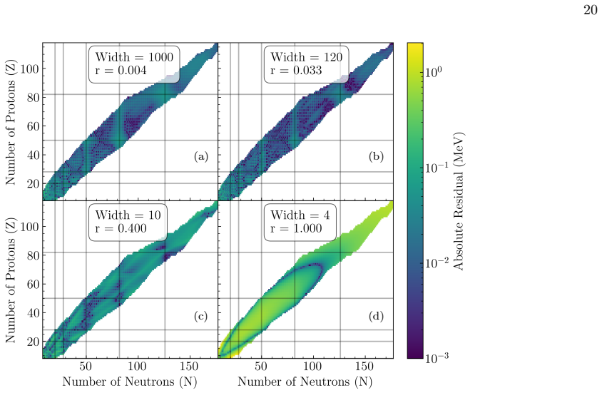
On the paper's own terms, the central discovery is that the field-theoretic criticality analysis of neural networks works as a predictive tool for a real nuclear-physics network. For a two-input ReLU network trained with SGD on AME2020 binding energies, critical initialization ($C_W=2$, $C_b=0$) leaves the pre-training output variance constant with depth while the excess kurtosis grows linearly in $\ell_{\text{out}}$, in agreement with recursion relations that treat the output distribution's action as an expansion in $r=\ell_{\text{out}}/n$; above or below criticality the variance explodes or vanishes. With critical initialization and critical training (layer-dependent learning rates scaled by depth and width), the networks reach the lowest MAE loss and a best binding-energy RMSD of about $1.9$ MeV, and the theoretical optimum ratio $r^*=0.034$ from Eq.~(50) lines up with the measured minimum at $r=0.033$. The paper also finds that Softplus, lacking a critical fixed point because $\sigma(0)\neq 0$, is more prone to exploding or vanishing variance, and that replacing SGD with the adaptive Adam optimizer removes the signature of criticality while giving somewhat better fits ($\sim 1.2$ MeV).
Load-bearing premise
The paper's evidence that critical training is superior rests on how the comparison runs were set up: the non-critical runs used learning rates averaged from the critical network, and no search over non-critical learning rates was done to see if they could match the critical results.
Editorial extensions
If this is right
- For feed-forward networks with activations satisfying $\sigma(0)=0$ and $\sigma'(0)\neq0$, critical initialization and critically scaled SGD learning rates remove the exploding/vanishing gradient problem without adaptive optimizers.
- The aspect-ratio formula $r^*$ gives a concrete, non-empirical choice of width for a given depth; for the two-input binding-energy network (depth 4, output width 1) it predicts $n\approx 115$, matching the observed RMSD minimum.
- Vanishing or exploding pre-training variance and non-linear kurtosis growth diagnose which activations (e.g., Softplus) will be unstable and less expressive in deep networks.
- Critical training with plain SGD on binding energies reaches about 1.9 MeV, within a small factor of the roughly 1.2 MeV Adam result, showing criticality can nearly close the gap to adaptive optimizers.
- Networks with $r$ above $r^*$ enter a chaotic regime with bimodal RMSD distributions and frequent training failures, giving a quantitative boundary for architecture search.
Reading between the lines
- If the criticality picture generalizes, architecture search for nuclear-physics ANNs could be replaced by solving recursion relations: fix depth, choose width from $r^*$, initialize at criticality, and scale learning rates; this is testable on other mass models or emulators.
- The paper leaves untested whether non-critical networks with independently tuned global learning rates perform as well as CICT; sweeping those rates would isolate whether criticality or the comparison protocol drives the observed gain.
- The four-input network's failure to match the reference Adam-trained result with critical prescriptions suggests the criticality analysis captures only part of what determines performance as inputs and features grow, pointing toward the need for RG flows that include input correlations.
- Because the criticality conditions are $\sigma(0)=0$ and $\sigma'(0)\neq0$, one could test Softplus shifted by $-\log 2$ to restore $\sigma(0)=0$ and check whether its depth stability and expressivity then match ReLU.
Editorial analysis
A structured set of objections, weighed in public.
Referee Report
Summary. The paper applies artificial neural network field theory (ANNFT), as developed by Roberts, Yaida, and collaborators, to a two-input, one-output feedforward ANN trained on AME2020 nuclear binding energies. It first validates the pre-training predictions of ANNFT: final-layer output distributions approach Gaussians as width grows, the ReLU variance recursion has a critical fixed point at C_W=2, C_b=0, and the excess kurtosis grows linearly with depth at criticality. It then tests training prescriptions with stochastic gradient descent, comparing critical initialization/critical training (CICT), critical initialization/non-critical training (CINT), and non-critical/non-critical training (NINT). The authors report that CICT achieves the lowest MAE loss and best binding-energy RMSD of about 1.9 MeV, and they claim an ANNFT prediction r*=0.034 for the optimal depth-to-width ratio that matches the observed minimum in the RMSD versus r curve at r=0.033. The paper closes by noting that Adam outperforms the critically tuned SGD networks, which the authors interpret as obscuring the criticality analysis.
Significance. If the central claims hold, the paper would provide a valuable, non-empirical route to architecture and hyperparameter selection for nuclear-physics ANNs, going beyond the usual black-box tuning. The strongest part of the paper is Sec. III: the variance and excess-kurtosis recursions are tested against simulations in a genuinely parameter-free way (using only G(0) and V(0)=0 as inputs), and the agreement shown in Figs. 6 and 7 is convincing. The comparison of critical versus non-critical initialization for ReLU and Softplus is also clearly presented. The training study in Sec. IV addresses a practically important question, but two load-bearing issues—the arithmetic inconsistency in the r* prediction and the construction of the non-critical training baseline—currently prevent the paper from supporting its headline quantitative claims.
major comments (4)
- [Sec. IV, Eq. (50) and Fig. 13] Eq. (50) is internally inconsistent with the quoted numerical value. With n_lout=1 and ν=5, the formula gives r* = (4/23)^(1/5) ≈ 0.705, not 0.034 as stated in the text and drawn in Fig. 13. The value 0.034 would require an exponent close to 2. This is a load-bearing discrepancy because the claimed quantitative match between ANNFT and the observed RMSD minimum at r=0.033 is one of the paper's central results. The authors must correct Eq. (50) (or the definition of ν, or the quoted value), and verify the formula against Appendix A of Ref. [8]; otherwise the observed minimum cannot be presented as validation of the ANNFT r* prediction.
- [Sec. IV, paragraph after Eq. (39), Figs. 8 and 9] The superiority of CICT over CINT and NINT is not established by the current protocol. The non-critical baselines use a single global SGD learning rate obtained by averaging the layer-dependent critical learning rates of the corresponding CICT network. This compares critical training against a particular averaged schedule, not against non-critical training with its own reasonably tuned learning rate. To support the claim that critical tuning, rather than the choice of comparison rates, drives the improvement, the authors should sweep or otherwise tune the non-critical learning rates (or compare against standard global SGD choices) and show that CICT remains superior.
- [Sec. IV, Table I and Fig. 13] Even setting aside the arithmetic error, the data provide only weak statistical support for the specific value of r*. The mean RMSD at r=0.0348 (width 115) is 2.5392 ± 0.2326 MeV, and at r=0.0333 (width 120) it is 2.5250 ± 0.2221 MeV; the difference is much smaller than one standard deviation. The presence of a broad minimum is clear, but the paper should not claim a precise quantitative confirmation of the ANNFT r* value without either tighter statistics or an explicit statement of the uncertainty in the location of the observed minimum.
- [Sec. IV, final paragraph] The paper states that a four-input network 'exhibited the same initialization and training behavior presented in Secs. III and IV,' but then reports that the critical four-input network could not match the RMSD of Ref. [6]'s optimized network and that even a reproduction of Ref. [6]'s architecture and hyperparameters did not reproduce its RMSD. This is a significant caveat for the generality of the conclusions, and it should be discussed more explicitly rather than left as a closing remark. In particular, the authors should indicate whether the failure is due to non-critical hyperparameters in Ref. [6], to the input representation, or to other implementation differences.
minor comments (5)
- [Fig. 14 caption] The caption says 'r=1 in Fig. 14(c) shows poor learning,' but the fourth panel is labeled (d); this should be corrected.
- [Figs. 11 and 12 captions] The captions contain the typo 'pre-taining' instead of 'pre-training'.
- [Conclusion, first paragraph] The word 'protoypical' should be 'prototypical'; the Fig. 13 caption also contains 'mininum' for 'minimum'.
- [Sec. IV, first paragraph of training comparison] The text says CICT networks use the critically scaled learning rates from Eq. (39), but Eq. (38) gives the ReLU rates and Eq. (39) gives the Tanh rates; the sentence should refer to both equations.
- [General] A data and code availability statement is missing. Given the paper's emphasis on reproducible validation of theoretical predictions, the authors should state where the AME2020 data, preprocessing details, and training code can be obtained.
Circularity Check
No circularity found: ANNFT predictions are externally sourced and clearly separated from empirical recursions; the Eq. (50) arithmetic issue is a correctness problem, not a circular step.
full rationale
The paper does not exhibit circularity in the senses defined by the checklist. The criticality conditions (ReLU C_W=2, C_b=0), the variance and excess-kurtosis recursion relations, and the r* formula are taken from the external ANNFT literature (Refs. [7-10]) rather than fitted to the AME2020 outputs, so the Sec. III and IV validations are tests against an independent theory. In Figs. 6 and 7 the paper explicitly distinguishes theory-only recursion (starting from G(0) and V(0)=0) from data-based recursion (starting from measured G(1) and V(1)), so those comparisons are not self-definitional. The training comparison uses a global CINT/NINT learning rate obtained by averaging the layer-dependent CICT rates; this is a possible baseline-fairness weakness, but it is not a constructional equivalence or a fitted-parameter-as-prediction, so it does not count as circularity under the hard rules. The r* = 0.034 claim is internally inconsistent: substituting n_lout=1 and nu=5 into Eq. (50) gives (4/23)^(1/5) approximately 0.705, not 0.034, so the claimed match with the observed minimum at r = 0.033 is unsupported as printed; this is an arithmetic/transcription error or a formula-usage issue, not a circular derivation. No self-citation is load-bearing, and no uniqueness or ansatz is imported from the present authors' own prior work.
Assumptions & free parameters
free parameters (4)
- Initialization weight variance CW for ReLU networks =
critical value 2.0 (also tested 1.0 and 3.0); Cb=0
- Unscaled learning rate constants \tilde\lambda_W, \tilde\lambda_b =
not specified in the paper
- Two-phase learning rate schedule switch epoch =
5000 epochs
- RMSD exclusion thresholds in performance statistics =
>= 30 MeV omitted in Fig. 13; > 100 MeV or NaN excluded in Table I
assumptions (6)
- standard math Central limit theorem: preactivations in a layer become Gaussian as width n goes to infinity for i.i.d. mean-zero weights and biases
- domain assumption The ratio r = depth/width is a small expansion parameter controlling non-Gaussian corrections
- domain assumption Trained output can be Taylor expanded about initialized parameters with truncation at third order
- domain assumption Criticality condition for ReLU: CW = 2 with Cb = 0 yields a variance fixed point
- domain assumption Optimal aspect-ratio formula r* = (4/(20+3 n_lout))^(1/nu) from Ref [8]
- domain assumption The learning-rate scaling formulas Eq. (38)-(39) for ReLU and Tanh are correct critical training prescriptions
Cite this review
Pith. "Pith review of Criticality analysis of nuclear binding energy neural networks." pith.science (2026). https://pith.science/paper/STFWRCM4
@misc{pith2026250801001,
  author       = {Pith},
  title        = {Pith review of: Criticality analysis of nuclear binding energy neural networks},
  year         = {2026},
  howpublished = {\url{https://pith.science/paper/STFWRCM4}},
  note         = {Machine review of arXiv:2508.01001}
}
read the original abstract
Machine learning methods, in particular deep learning methods such as artificial neural networks (ANNs) with many layers, have become widespread and useful tools in nuclear physics. However, these ANNs are typically treated as ``black boxes'', with their architecture (width, depth, and weight/bias initialization) and the training algorithm and parameters chosen empirically by optimizing learning based on limited exploration. We test a non-empirical approach to understanding and optimizing nuclear physics ANNs by adapting a criticality analysis based on renormalization group flows in terms of the hyperparameters for weight/bias initialization, training rates, and the ratio of depth to width. This treatment utilizes the statistical properties of neural network initialization to find a generating functional for network outputs at any layer, allowing for a path integral formulation of the ANN outputs as a Euclidean statistical field theory. We use a prototypical example to test the applicability of this approach: a simple ANN for nuclear binding energies. We find that with training using a stochastic gradient descent optimizer, the predicted criticality behavior is realized, and optimal performance is found with critical tuning. However, the use of an adaptive learning algorithm leads to somewhat superior results without concern for tuning and thus obscures the analysis. Nevertheless, the criticality analysis offers a way to look within the black box of ANNs, which is a first step towards potential improvements in network performance beyond using adaptive optimizers.
Figures


Figures from the paper (11 more)


Reference graph
Works this paper leans on
-
[8]
D. A. Roberts, S. Yaida, and B. Hanin,The Principles of Deep Learning Theory(Cambridge University Press,
-
[6]
Nuclear binding energies in artificial neural networks
L.-X. Zeng, Y.-Y. Yin, X.-X. Dong, and L.-S. Geng, Phys. Rev. C 109, 034318 (2024), arXiv:2210.02906 [nucl-th]
work page Pith review arXiv 2024
-
[1]
A. Boehnlein, M. Diefenthaler, N. Sato, M. Schram, V. Ziegler, C. Fanelli, M. Hjorth-Jensen, T. Horn, M. P. Kuchera, D. Lee, W. Nazarewicz, P. Ostroumov, K. Orginos, A. Poon, X.-N. Wang, A. Scheinker, M. S. Smith, and L.-G. Pang, Rev. Mod. Phys. 94, 031003 (2022), arXiv:2112.02309 [nucl-th]
arXiv 2022
-
[2]
G. Carleo, I. Cirac, K. Cranmer, L. Daudet, M. Schuld, N. Tishby, L. Vogt-Maranto, and L. Zdeborová, Re- views of Modern Physics 91 (2019), 10.1103/revmod- phys.91.045002
doi:10.1103/revmod- 2019
-
[3]
A. M. Deiana, N. Tran, J. Agar, M. Blott, G. Di Guglielmo, J. Duarte, P. Harris, S. Hauck, M. Liu, M. S. Neubauer, J. Ngadiuba, S. Ogrenci- Memik, M. Pierini, T. Aarrestad, S. Bähr, J. Becker, A.-S. Berthold, R. J. Bonventre, T. E. Müller Bravo, M. Diefenthaler, Z. Dong, N. Fritzsche, A. Gholami, E. Govorkova, D. Guo, K. J. Hazelwood, C. Herwig, B. Khan, ...
-
[4]
Precise neural network predictions of energies and radii from the no-core shell model
T. Wolfgruber, M. Knöll, and R. Roth, Phys. Rev. C 110, 014327 (2024), arXiv:2310.05256 [nucl-th]
work page Pith review arXiv 2024
- [5]
-
[7]
D. A. Roberts, (2021), arXiv:2104.00008 [hep-th]
arXiv 2021
Show all 44 references
-
[9]
Halverson, A
J. Halverson, A. Maiti, and K. Stoner, Mach. Learn. Sci. Tech. 2, 035002 (2021), arXiv:2008.08601 [cs.LG]
2021 arXiv
-
[10]
Halverson, (2021), arXiv:2112.04527 [hep-th]
J. Halverson, (2021), arXiv:2112.04527 [hep-th]
2021 arXiv
-
[11]
A correspondence between random neural networks and statistical field theory,
S. S. Schoenholz, J. Pennington, and J. Sohl-Dickstein, “A correspondence between random neural networks and statistical field theory,” (2017), arXiv:1710.06570 [stat.ML]
2017 arXiv
-
[12]
Cohen, O
O. Cohen, O. Malka, and Z. Ringel, Phys. Rev. Res.3, 023034 (2021)
2021
-
[13]
Bachtis, G
D. Bachtis, G. Aarts, and B. Lucini, Phys. Rev. D103, 074510 (2021), arXiv:2102.09449 [hep-lat]
2021 arXiv
-
[14]
Erdmenger, K
J. Erdmenger, K. T. Grosvenor, and R. Jefferson, Sci- Post Phys. 12, 041 (2022), arXiv:2107.06898 [hep-th]
2022 arXiv
-
[15]
Erbin, V
H. Erbin, V. Lahoche, and D. O. Samary, Mach. Learn. Sci. Tech.3, 015027 (2022), arXiv:2108.01403 [hep-th]
2022 arXiv
- [16]
-
[17]
Bishop, Pattern recognition and machine learning, Vol
C. Bishop, Pattern recognition and machine learning, Vol. 4 (Springer New York, 2006)
2006
-
[18]
Y. S. Abu-Mostafa, M. Magdon-Ismail, and H.-T. Lin, Learning From Data(AMLBook, 2012)
2012
-
[19]
K. P. Murphy,Machine Learning: A Probabilistic Per- spective (The MIT Press, 2012)
2012
-
[20]
Mehta, M
P. Mehta, M. Bukov, C.-H. Wang, A. G. Day, C. Richard- son, C.K.Fisher, andD.J.Schwab,Physicsreports 810, 1 (2019)
2019
-
[21]
C. M. Bishop and H. Bishop,Deep learning: Foundations and concepts(Springer, 2024)
2024
-
[22]
Abdulkadirov, P
R. Abdulkadirov, P. Lyakhov, and N. Nagornov, Math- ematics 11 (2023), 10.3390/math11112466
2023 doi
-
[23]
On the variance of the adaptive learning rate and beyond,
L. Liu, H. Jiang, P. He, W. Chen, X. Liu, J. Gao, and J. Han, “On the variance of the adaptive learning rate and beyond,” (2021), arXiv:1908.03265 [cs.LG]
2021 arXiv
-
[24]
Priors for infinite networks,
R. M. Neal, “Priors for infinite networks,” inBayesian Learning for Neural Networks(Springer New York, New York, NY, 1996) pp. 29–53
1996
-
[25]
C. K. I. Williams, inNIPS (1996)
1996
-
[26]
Deep neural networks as gaussian processes,
J. Lee, Y. Bahri, R. Novak, S. S. Schoenholz, J. Penning- ton, and J. Sohl-Dickstein, “Deep neural networks as gaussian processes,” (2018), arXiv:1711.00165 [stat.ML]
2018 arXiv
-
[27]
Gaussian process be- haviour in wide deep neural networks,
A. G. de G. Matthews, M. Rowland, J. Hron, R. E. Turner, and Z. Ghahramani, “Gaussian process be- haviour in wide deep neural networks,” (2018), arXiv:1804.11271 [stat.ML]
2018 arXiv
-
[28]
Jacot, F
A. Jacot, F. Gabriel, and C. Hongler, Proceedings of the 53rd Annual ACM SIGACT Symposium on Theory of Computing (2018)
2018
-
[29]
Finite depth and width corrections to the neural tangent kernel,
B. Hanin and M. Nica, “Finite depth and width corrections to the neural tangent kernel,” (2019), arXiv:1909.05989 [cs.LG]
2019 arXiv
-
[30]
Quasi-equivalence of width and depth of neural networks,
F.-L. Fan, R. Lai, and G. Wang, “Quasi-equivalence of width and depth of neural networks,” (2022)
2022
-
[31]
Álvarez López, A
A. Álvarez López, A. Slimane, and E. Zuazua, Neural Networks 180 (2024), 10.2139/ssrn.4753244
2024 doi
-
[32]
Radhakrishnan, M
A. Radhakrishnan, M. Belkin, and C. Uhler, Proceed- ings of the National Academy of Sciences 120 (2023), 10.1073/pnas.2208779120
2023 doi
-
[33]
Width is less important than depth in relu neural networks,
G. Vardi, G. Yehudai, and O. Shamir, “Width is less important than depth in relu neural networks,” (2022), arXiv:2202.03841
2022 arXiv
-
[34]
Do wide and deep networks learn the same things? uncovering how neural network representations vary with width and depth,
T. Nguyen, M. Raghu, and S. Kornblith, “Do wide and deep networks learn the same things? uncovering how neural network representations vary with width and depth,” (2020), arXiv:2010.15327
2020 arXiv
-
[35]
Neural tangent kernel: Convergence and generalization in neural net- works,
A. Jacot, F. Gabriel, and C. Hongler, “Neural tangent kernel: Convergence and generalization in neural net- works,” (2020)
2020
-
[36]
The neural tangent kernel,
S. Prince, “The neural tangent kernel,” (2024)
2024
-
[37]
Some math behind neural tangent kernel,
L. Weng, “Some math behind neural tangent kernel,” (2022)
2022
-
[38]
Fast finite width neural tangent kernel,
R. Novak, J. Sohl-Dickstein, and S. S. Schoenholz, “Fast finite width neural tangent kernel,” (2022)
2022
-
[39]
Glorot, A
X. Glorot, A. Bordes, and Y. Bengio, inProceedings of the Fourteenth International Conference on Artificial In- telligence and Statistics, Proceedings of Machine Learn- ing Research, Vol. 15, edited by G. Gordon, D. Dunson, and M. Dudík (PMLR, Fort Lauderdale, FL, USA, 2011) p...
2011
-
[40]
A. K. Bhoi, P. K. Mallick, C.-M. Liu, and V. E. Balas, eds., Bio-inspired Neurocomputing, Vol. 903 (Springer Singapore, 2021)
2021
-
[41]
Activa- tion functions in deep learning: A comprehensive survey and benchmark,
S. R. Dubey, S. K. Singh, and B. B. Chaudhuri, “Activa- tion functions in deep learning: A comprehensive survey and benchmark,” (2022), arXiv:2109.14545 [cs.LG]
2022 arXiv
-
[42]
Virtanen, R
P. Virtanen, R. Gommers, T. E. Oliphant, M. Haber- land, T. Reddy, D. Cournapeau, E. Burovski, P. Pe- terson, W. Weckesser, J. Bright, S. J. van der Walt, M. Brett, J. Wilson, K. J. Millman, N. Mayorov, A. R. J. Nelson, E. Jones, R. Kern, E. Larson, C. J. Carey, İ. Po- lat, Y....
2020
-
[43]
Adam: Amethodforstochastic optimization,
D.P.KingmaandJ.Ba,“Adam: Amethodforstochastic optimization,” (2017), arXiv:1412.6980 [cs.LG]
2017 arXiv
-
[2022]
arXiv:2106.10165 [cs.LG]
Reviewed August 6, 2026 · model on record in the stance chip above.
Discussion (0). Sign in to comment.