REVIEW 3 major objections 5 minor 226 references
A carefully structured neural field, fit at test time to raw smartphone burst captures, can recover accurate depth, separate image layers, and stitch panoramas without labeled data, pre-processing, or learned priors.
Reviewed by Pith at T0; open to challenge. T0 means a machine referee read the full paper against a public rubric. the ladder, T0–T4 →
Fitting neural fields directly to raw phone bursts reconstructs depth, separates reflections and occluders, and stitches panoramas, outperforming the compared baselines on the thesis's benchmarks.
T0 review reviewed 2026-08-05 challenge →
load-bearing objection A well-written compilation of three strong peer-reviewed papers, but not new research and the abstract overclaims what the body honestly concedes. the 3 major comments →
Neural Field Representations of Mobile Computational Photography
The pith
A machine-rendered reading of the paper's core claim, the machinery that carries it, and where it could break.
The reading
Core claim
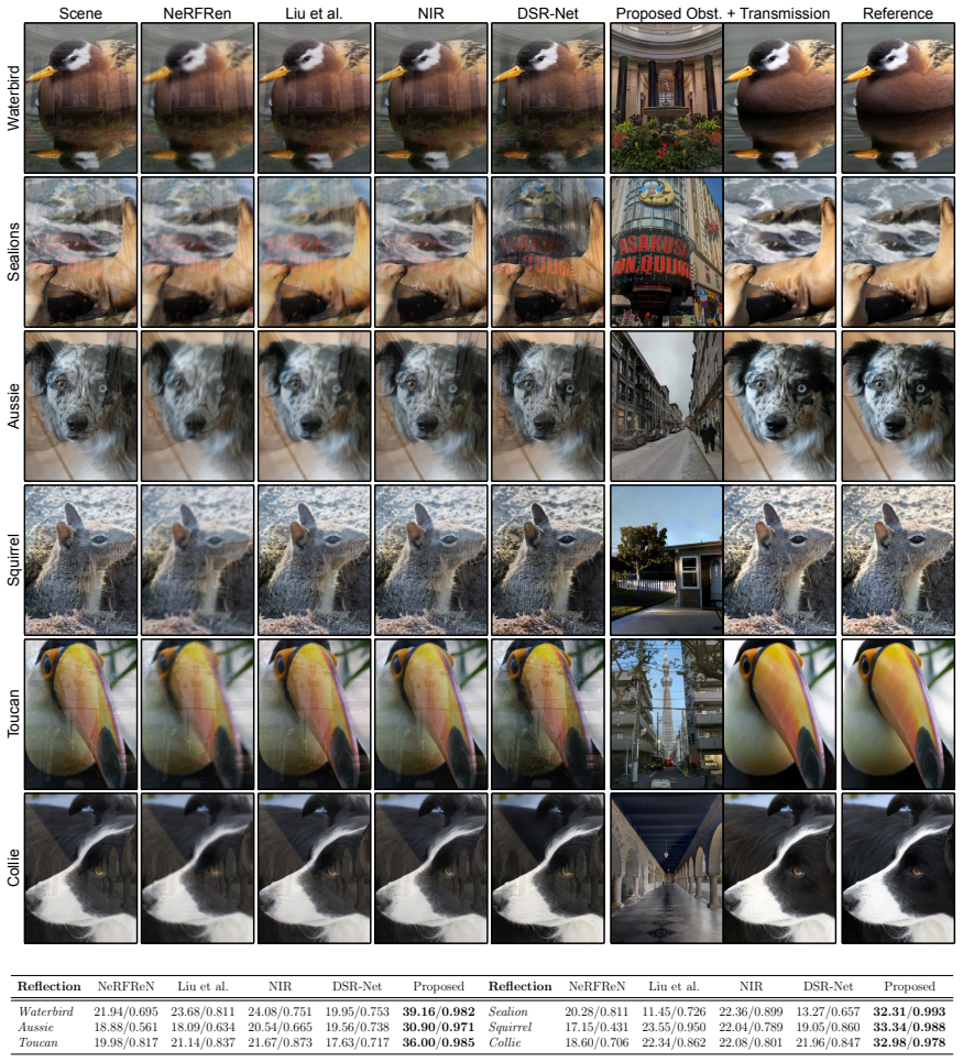
The central claim is that carefully designed neural field models can compactly represent complex geometry and lighting from in-the-wild mobile photography, outperforming state-of-the-art methods without complex pre-processing, labeled ground truth, or machine learning priors. For micro-baseline depth, a plane-plus-offset implicit depth model fit jointly with an implicit image and a low-dimensional motion model recovers geometrically accurate depth from a two-second, 42-frame RAW burst. For layer separation, a two-plane alpha-composited model whose flows are controlled by neural spline fields separates occluders, reflections, shadows, and haze from background content. For image stitching, a n
What carries the argument
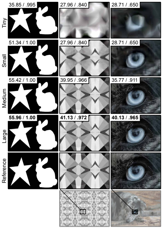
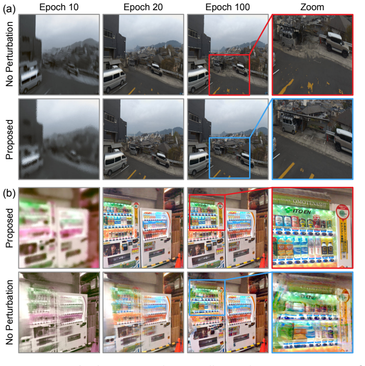
The central machinery is the neural field itself, parameterized with multiresolution hash encodings for fast training and controllable spatial frequency. Depth uses a forward-projection RGB-D model with a learned planar background plus offset; layer separation uses backward-projected rays through two alpha-composited planes, with flows given by neural spline fields whose temporal smoothness is built into a cubic Hermite spline rather than regularized; image stitching relies on a ray-sphere intersection model with a view-dependent ray-offset network and a view-dependent color network. In each case the model's structure—plane regularization, spline parameterization, or a two-stage training sch
Load-bearing premise
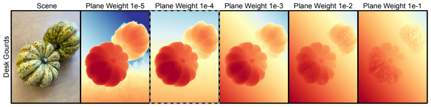
The depth recovery assumes the scene decomposes into a single static background plane plus small foreground depth offsets, and that a hand-tuned regularization weight picks the geometrically true depth among many photometrically equivalent solutions.
What would settle it
Capture a long-burst of a scene whose background is a close, curved, non-planar surface with no dominant plane. If the fitted depth collapses to a plane or follows image texture instead of true geometry—the paper's own Sec. 2.9 concedes the plane is often 'more akin to a segmentation mask than depth'—the central claim that parallax alone recovers geometrically accurate depth from micro-baseline data is falsified.
If this is right
- If the depth claims hold, ordinary unstabilized phone captures become a viable source of dense, geometrically consistent depth without dedicated depth sensors or learned monocular priors.
- Layer separation from a burst could turn reflection and occlusion removal into a standard post-capture operation, with the alpha matte produced automatically.
- Neural spline fields provide a controllable flow representation that may generalize to other multi-frame fusion tasks such as denoising, deblurring, and video segmentation.
- The neural light sphere model could make interactive panorama viewing—rather than static stitched images—a practical phone feature, with real-time rendering and modest model size.
- The test-time optimization paradigm suggests that emerging sensors, such as hyperspectral or polarization imagers, could be handled without retraining on large datasets, by fitting the same kinds of self-regularized models to their raw data.
Where Pith is reading between the lines
- The plane-plus-offset depth decomposition, which the paper itself notes is often a segmentation mask as much as a depth map, could be exploited more directly: the depth offset and plane can serve jointly for matting and compositing, a connection the thesis shows but leaves as an auxiliary application.
- The dependence on hand-tuned hyperparameters (plane weight, encoding sizes, spline controls) hints at a future where these are selected automatically per scene, since the thesis demonstrates per-scene optimal settings differ.
- The success of the spline flow representation on small-motion bursts suggests it could be adapted to video compression or editable video layers, where the spline's built-in temporal continuity would avoid flicker artifacts.
- Because the methods fit raw sensor data without learned priors, they could be applied to non-smartphone imaging platforms—microscopes, telescopes, drones—by providing the appropriate projection and motion models, though the thesis stops short of demonstrating this.
Editorial analysis
A structured set of objections, weighed in public.
Referee Report
Summary. The dissertation proposes neural field models fitted at test time to raw smartphone burst and panoramic captures, addressing three tasks: micro-baseline depth estimation (Ch. 2), layer separation for occlusion/reflection/shadow removal (Ch. 3), and panoramic stitching with view synthesis (Ch. 4). The central claim is that carefully designed, self-regularized neural field representations, fit directly to raw sensor data by stochastic gradient descent, outperform state-of-the-art methods without labeled data, learned priors, or complex preprocessing. Each chapter presents a forward model, a neural field parameterization, real and synthetic evaluations, and an extensive set of qualitative results and ablations. The thesis is honest about many failure modes: dynamic, textureless, distant, translucent, and reflective scenes are documented in Sec. 2.10 and Fig. 2.16, and Sec. 2.9 explicitly concedes that the plane component often behaves as a segmentation mask rather than measured depth.
Significance. If the central thesis is correct, it would establish test-time neural field fitting as a broadly applicable alternative to supervised or pipeline-based computational photography, with the practical appeal of operating on raw captures from commodity phones. The work has several genuine strengths: it ships real captured datasets, records raw sensor data with gyroscope/metadata, provides open-source capture tools and project pages, validates depth on structured-light ground-truth scans (Fig. 2.7), and includes detailed ablations of encoding size, regularization, frame count, and motion scale. The three method chapters each introduce a compact representation (depth-on-a-plane, neural spline fields, neural light sphere) that is plausible and, within the tested conditions, often qualitatively superior to baselines. However, the abstract-level claim about being 'without... machine learning priors' and generally superior is significantly stronger than what the internal evidence supports, because the depth objective is shown to be degenerate and the selected solution is chosen by hand-tuned geometric and optimization priors. The contribution is still valuable as a demonstration of what thes
major comments (3)
- [Sec. 2.5, Eq. (2.7), Eqs. (2.10)-(2.13), Fig. 2.11, Sec. 2.9] The central depth claim is not supported by the paper's own evidence. Fig. 2.11 shows two radically different depth maps with identical reprojection error, and Sec. 2.9 concedes that the plane component is often 'more akin to a segmentation mask than depth.' The depth model in Eq. (2.7) imposes a single plane plus ReLU offset, and the objective in Eqs. (2.10)-(2.13) with alpha_p = 1e-4 selects the solution among photometrically equivalent ones. Thus for textureless, distant, or non-planar regions, the recovered depth is not measured from parallax but assigned by a hand-tuned regularizer. This directly undercuts the abstract's claim of recovering depth 'without... machine learning priors' and 'self-regularized models.' The authors should reframe the depth contribution as prior-guided affine depth estimation, provide sensitivity of alpha_p across a broader range of scenes, and avoid claimi
- [Sec. 2.11 and Sec. 3.6] Both synthetic benchmarks are generated under the same geometric assumptions as the proposed methods. In Sec. 2.11, synthetic scenes place a textured object in front of a tilted background plane, use the hand-shake paths measured by the authors' prior app, and render with the same small-angle camera model. In Sec. 3.6, transmission and obstruction planes are placed at Pi_z depths, composited with the same planar model and the same hand-shake data. Because the synthetic data is a special case of the model family, high quantitative scores there do not validate generalization to scenes that violate the plane-plus-offset or two-plane assumptions. The qualitative real-data results are useful, but the 'outperform SOTA' claim is not yet established for general in-the-wild captures.
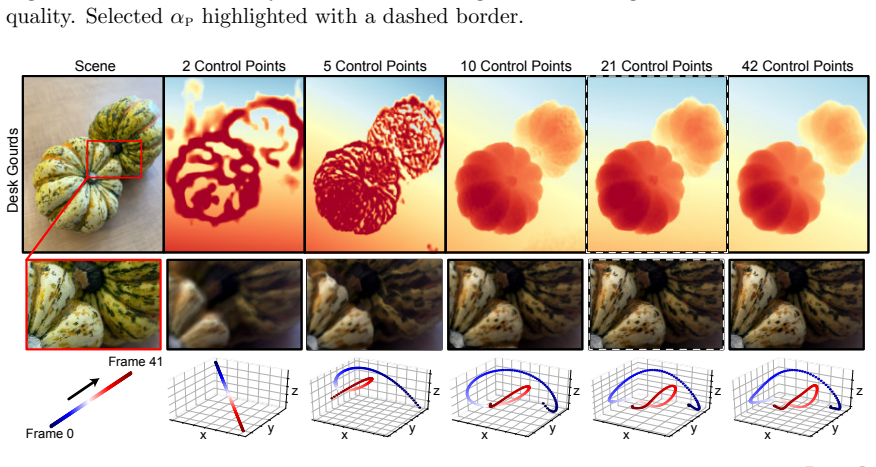
- [Ch. 3, Table 3.2 and Sec. 3.6] The layer separation chapter relies on task-specific configurations that are manually selected per application: flow encoding size, number of spline control points, plane depths, alpha regularization weight, and even separate columns for occlusion, reflection, shadow, and dehazing. The authors note these are 'not prescriptive' and that all neural scene fitting has per-scene parameters, but this undermines the thesis-level claim of a single 'well-constructed, self-regularized model.' To support the strong claim, the paper would need either a demonstration that one fixed configuration works across all tasks, or a clear admission that the method requires manual per-task or per-scene tuning.
minor comments (5)
- [Abstract and Ch. 1] The phrase 'without relying on... machine learning priors' is technically about learned priors, but the method relies on hand-designed geometric priors (single-plane, spline smoothness, hash-grid resolution limits, regularization weights). Consider rewording to 'without learned priors or labeled data' and explicitly acknowledge hand-crafted regularizers.
- [Sec. 2.5, Eq. (2.10)] The notation L = L_d + alpha_p (L_p/L_d) R is confusing because L_p and L_d are already defined as losses; the ratio may be intended as a per-sample weighting. Please clarify the indexing and whether the ratio is taken pointwise or as a scalar.
- [Sec. 3.3.1] The claim that the neural spline field 'produces temporally consistent flow with no regularization' is supported mainly by the qualitative comparison in Fig. 3.2. Quantitative flow error against a reference estimator would strengthen the claim.
- [Sec. 4.4.1] The comparison to traditional image stitching is presented visually and with limited metrics. Since the chapter claims 50 FPS rendering and 80 MB model size, a benchmark table of runtime, memory, and PSNR against classic stitchers would help.
- [Throughout] There are minor typographical and formatting errors (e.g., 'frament' in Sec. 2.6, 'RA W' spacing, and the duplicated equation numbers in Ch. 4). These do not affect the science but should be cleaned up.
Circularity Check
Central derivations are self-contained, but the synthetic validation scenes are generated from the same plane/alpha-composite forward models, creating a partial validation loop.
specific steps
-
other
[Sec. 3.6 Synthetic Data Generation; cf. Sec. 2.11 Synthetic Evaluation]
"These are simulated as 3D planes in space at depths Π o z and Π t z respectively – Π o z < Π t z for occluders and Π o z > Π t z for reflectors – and apply a random tilt to the planes with angle θ∈[−20 ◦,20 ◦]. To generate realistic camera motion, we record samples of natural hand tremor with a pose-capture application built on the Apple ARKit library [42]. We then apply this motion path to a projective camera model, re-sample the image planes, and alpha-composite the outputs to produce the simulated burst stack."
The synthetic ground truth is produced by the same forward model the method optimizes: two image planes at depths Π_z, re-sampled by a projective camera with hand-shake motion, then alpha-composited — matching Eq. 3.10 (ĉ=(1−α)c_t+αc_o) and the plane/flow model of Sec. 3.3.2. Similarly, the Ch2 synthetic scenes (Sec. 2.11) are a plane background plus offset objects, matching the plane-plus-offset depth model of Eq. 2.7, with motion from the authors' own prior hand-shake capture. Thus 'near ground truth' reconstruction on these scenes is guaranteed up to optimization error by construction; these benchmarks cannot independently confirm the core plane/alpha-composite assumptions. The real-data comparisons (structured-light scans, tripod reference captures) remain external, so this is a partia
full rationale
The core derivations in Chapters 2–4 are not circular: depth, layer, and panorama models are fit to raw burst/panoramic data via photometric losses with explicit, disclosed regularizers (α_p, η_α), and the depth degeneracy is acknowledged in Fig. 2.11 and Sec. 2.9 rather than hidden. Real-world validation includes independent structured-light scans (Sec. 2.6) and tripod-reference captures (Sec. 3.4), so the central claims have external support. However, the synthetic validation loops are a genuine weakness: the Ch2 synthetic long-bursts place scanned objects in front of a plane and render with the authors' own hand-shake paths, exactly the plane-plus-offset scene model of Eq. 2.7; the Ch3 synthetic bursts are generated by alpha-compositing two planes with the same projective and motion model, exactly Eq. 3.10. Success on these scenes partly reflects that the data was constructed from the method's own assumptions, so the synthetic benchmarks cannot independently validate the plane/alpha-composite priors. This is a partial circularity in validation, not in the derivation of the methods, and the independent real-data results keep the central claims from being reduced to the model's own construction. The self-citations to Chugunov et al. [42] supply empirical hand-shake measurements rather than unverified uniqueness theorems, so they are not load-bearing in a circular way.
Axiom & Free-Parameter Ledger
free parameters (9)
- plane regularization weight α_p =
1e-4
- rotation offset weight η_r =
1e-4 (Ch. 2), 1e-3 (Ch. 4)
- coarse-to-fine sweep constants k_min, k_max =
-100, 200
- Bezier control points N_c =
21 per curve
- depth hash encoding L_γd, N_max, T_γd =
8 levels, max 128, table 2^14
- per-task encoding sizes and loss weights (Ch. 3) =
occlusion η_α=0.02; reflection η_α=0.0; shadow η_α=2.0; flow sizes |h|=11 or 15; plane depths Π_z per task
- alpha temperature τ_σ =
not stated in available text
- ray perturbation weight η_p =
decayed to zero over stage 1
- NeuLS hash grids γ1, γ2 =
γ1: 8 levels, 4 to 112; γ2: 15 levels, 4 to 3145; table 2^19
axioms (9)
- domain assumption Static, Lambertian scene model with known intrinsics and pinhole projection
- ad hoc to paper Background is a single plane plus foreground offset
- ad hoc to paper Plane regularization resolves the photometric degeneracy
- domain assumption Common fate: obstructing and transmitted layers move differently and can be separated by two alpha-composited planes
- ad hoc to paper Spline parametrization with low-resolution encodings prevents flow overfitting without explicit regularization
- ad hoc to paper Ray-offset plus view-dependent color on a sphere explains parallax, motion, and lighting for panorama captures
- ad hoc to paper Synthetic validation data is built under the model's own geometric assumptions
- domain assumption RAW frames are linear with known black level and shading correction
- standard math Small-angle rotation approximation holds for hand tremor
Cite this review
Pith. "Pith review of Neural Field Representations of Mobile Computational Photography." pith.science (2026). https://pith.science/paper/E2AVE4YU
@misc{pith2026250805907,
  author       = {Pith},
  title        = {Pith review of: Neural Field Representations of Mobile Computational Photography},
  year         = {2026},
  howpublished = {\url{https://pith.science/paper/E2AVE4YU}},
  note         = {Machine review of arXiv:2508.05907}
}
read the original abstract
Over the past two decades, mobile imaging has experienced a profound transformation, with cell phones rapidly eclipsing all other forms of digital photography in popularity. Today's cell phones are equipped with a diverse range of imaging technologies - laser depth ranging, multi-focal camera arrays, and split-pixel sensors - alongside non-visual sensors such as gyroscopes, accelerometers, and magnetometers. This, combined with on-board integrated chips for image and signal processing, makes the cell phone a versatile pocket-sized computational imaging platform. Parallel to this, we have seen in recent years how neural fields - small neural networks trained to map continuous spatial input coordinates to output signals - enable the reconstruction of complex scenes without explicit data representations such as pixel arrays or point clouds. In this thesis, I demonstrate how carefully designed neural field models can compactly represent complex geometry and lighting effects. Enabling applications such as depth estimation, layer separation, and image stitching directly from collected in-the-wild mobile photography data. These methods outperform state-of-the-art approaches without relying on complex pre-processing steps, labeled ground truth data, or machine learning priors. Instead, they leverage well-constructed, self-regularized models that tackle challenging inverse problems through stochastic gradient descent, fitting directly to raw measurements from a smartphone.
Figures














Reference graph
Works this paper leans on
-
[1]
Defocus deblurring using dual-pixel data
Abdullah Abuolaim and Michael S Brown. Defocus deblurring using dual-pixel data. InEuropean Conference on Computer Vision, pages 111–126. Springer, 2020
2020
-
[2]
De-fencing and multi-focus fusion using markov random field and image inpainting.IEEE Access, 10:35992–36005, 2022
Hannan Adeel, Muhammad Mohsin Riaz, and Syed Sohaib Ali. De-fencing and multi-focus fusion using markov random field and image inpainting.IEEE Access, 10:35992–36005, 2022
2022
-
[3]
Pyramid methods in image processing.RCA engineer, 29(6):33– 41, 1984
Edward H Adelson, Charles H Anderson, James R Bergen, Peter J Burt, and Joan M Ogden. Pyramid methods in image processing.RCA engineer, 29(6):33– 41, 1984
1984
-
[4]
Interactive digital photomontage
Aseem Agarwala, Mira Dontcheva, Maneesh Agrawala, Steven Drucker, Alex Colburn, Brian Curless, David Salesin, and Michael Cohen. Interactive digital photomontage. InACM SIGGRAPH 2004 Papers, pages 294–302. 2004
2004
-
[5]
Panoramic video tex- tures
Aseem Agarwala, Ke Colin Zheng, Chris Pal, Maneesh Agrawala, Michael Co- hen, Brian Curless, David Salesin, and Richard Szeliski. Panoramic video tex- tures. InACM SIGGRAPH 2005 Papers, pages 821–827. 2005
2005
-
[6]
Nonrigid structure from motion in trajectory space.Advances in neural information processing systems, 21, 2008
Ijaz Akhter, Yaser Sheikh, Sohaib Khan, and Takeo Kanade. Nonrigid structure from motion in trajectory space.Advances in neural information processing systems, 21, 2008
2008
-
[7]
Video from stills: Lensless imaging with rolling shutter
Nick Antipa, Patrick Oare, Emrah Bostan, Ren Ng, and Laura Waller. Video from stills: Lensless imaging with rolling shutter. In2019 IEEE International Conference on Computational Photography (ICCP), pages 1–8. IEEE, 2019
2019
-
[8]
Learning neural light fields with ray-space embedding
Benjamin Attal, Jia-Bin Huang, Michael Zollh¨ ofer, Johannes Kopf, and Changil Kim. Learning neural light fields with ray-space embedding. InProceedings of the IEEE/CVF Conference on Computer Vision and Pattern Recognition, pages 19819–19829, 2022
2022
-
[9]
Matryodshka: Real-time 6dof video view synthesis using multi-sphere images
Benjamin Attal, Selena Ling, Aaron Gokaslan, Christian Richardt, and James Tompkin. Matryodshka: Real-time 6dof video view synthesis using multi-sphere images. InEuropean Conference on Computer Vision, pages 441–459. Springer, 2020. 136
2020
-
[10]
Explorable super resolution
Yuval Bahat and Tomer Michaeli. Explorable super resolution. InProceedings of the IEEE/CVF Conference on Computer Vision and Pattern Recognition, pages 2716–2725, 2020
2020
-
[11]
Depth-aware video frame interpolation
Wenbo Bao, Wei-Sheng Lai, Chao Ma, Xiaoyun Zhang, Zhiyong Gao, and Ming- Hsuan Yang. Depth-aware video frame interpolation. InProceedings of the IEEE/CVF Conference on Computer Vision and Pattern Recognition, pages 3703–3712, 2019
2019
-
[12]
Shape, illumination, and reflectance from shading.IEEE transactions on pattern analysis and machine intelligence, 37(8):1670–1687, 2014
Jonathan T Barron and Jitendra Malik. Shape, illumination, and reflectance from shading.IEEE transactions on pattern analysis and machine intelligence, 37(8):1670–1687, 2014
2014
-
[13]
Mip-nerf: A multiscale representa- tion for anti-aliasing neural radiance fields
Jonathan T Barron, Ben Mildenhall, Matthew Tancik, Peter Hedman, Ricardo Martin-Brualla, and Pratul P Srinivasan. Mip-nerf: A multiscale representa- tion for anti-aliasing neural radiance fields. InProceedings of the IEEE/CVF International Conference on Computer Vision, pages 5855–5864, 2021
2021
-
[14]
Zip-nerf: Anti-aliased grid-based neural radiance fields
Jonathan T Barron, Ben Mildenhall, Dor Verbin, Pratul P Srinivasan, and Peter Hedman. Zip-nerf: Anti-aliased grid-based neural radiance fields. In Proceedings of the IEEE/CVF International Conference on Computer Vision, pages 19697–19705, 2023
2023
-
[15]
Color imaging array.United States Patent 3,971,065, 1976
Bryce E Bayer. Color imaging array.United States Patent 3,971,065, 1976
1976
-
[16]
Om- niphotos: casual 360 vr photography.ACM Transactions on Graphics (TOG), 39(6):1–12, 2020
Tobias Bertel, Mingze Yuan, Reuben Lindroos, and Christian Richardt. Om- niphotos: casual 360 vr photography.ACM Transactions on Graphics (TOG), 39(6):1–12, 2020
2020
-
[17]
CRC press, 2021
Mario Bertero, Patrizia Boccacci, and Christine De Mol.Introduction to inverse problems in imaging. CRC press, 2021
2021
-
[18]
Deep burst super-resolution
Goutam Bhat, Martin Danelljan, Luc Van Gool, and Radu Timofte. Deep burst super-resolution. InProceedings of the IEEE/CVF Conference on Computer Vision and Pattern Recognition, pages 9209–9218, 2021
2021
-
[19]
Adabins: Depth estimation using adaptive bins
Shariq Farooq Bhat, Ibraheem Alhashim, and Peter Wonka. Adabins: Depth estimation using adaptive bins. InProceedings of the IEEE/CVF Conference on Computer Vision and Pattern Recognition, pages 4009–4018, 2021
2021
-
[20]
Color constancy using cnns
Simone Bianco, Claudio Cusano, and Raimondo Schettini. Color constancy using cnns. InProceedings of the IEEE conference on computer vision and pattern recognition workshops, pages 81–89, 2015
2015
-
[21]
Smartphone imaging technology and its applications.Advanced Optical Technologies, 10(3):145–232, 2021
Vladan Blahnik and Oliver Schindelbeck. Smartphone imaging technology and its applications.Advanced Optical Technologies, 10(3):145–232, 2021
2021
-
[22]
High-precision wafer- level optics fabrication and integration.Photonics Spectra, 2011
Jens Bliedtner, Andreas Gebhardt, and Uwe Schmidt. High-precision wafer- level optics fabrication and integration.Photonics Spectra, 2011. 137
2011
-
[23]
John Wiley & Sons, 2006
Mary L Boas.Mathematical methods in the physical sciences. John Wiley & Sons, 2006
2006
-
[24]
W. S. Boyle and G. E. Smith. Charge coupled semiconductor devices.Bell System Technical Journal, 49(4):587–593, 1970
1970
-
[25]
Brainard and Anya C
David H. Brainard and Anya C. Hurlbert. Colour vision: Understanding the- dress.Current Biology, 25(13):R551–R554, 2015
2015
-
[26]
Unprocessing images for learned raw denoising
Tim Brooks, Ben Mildenhall, Tianfan Xue, Jiawen Chen, Dillon Sharlet, and Jonathan T Barron. Unprocessing images for learned raw denoising. InProceed- ings of the IEEE/CVF conference on computer vision and pattern recognition, pages 11036–11045, 2019
2019
-
[27]
Automatic panoramic image stitching using invariant features.International journal of computer vision, 74:59–73, 2007
Matthew Brown and David G Lowe. Automatic panoramic image stitching using invariant features.International journal of computer vision, 74:59–73, 2007
2007
-
[28]
Photo statistics: How many photos are taken every day?, 2024
Matic Broz. Photo statistics: How many photos are taken every day?, 2024. Accessed: 2024-12-10
2024
-
[29]
A spatial processor model for object colour perception
Gershon Buchsbaum. A spatial processor model for object colour perception. Journal of the Franklin Institute, 310(1):1–26, 1980
1980
-
[30]
Unstructured lumigraph rendering
Chris Buehler, Michael Bosse, Leonard McMillan, Steven Gortler, and Michael Cohen. Unstructured lumigraph rendering. InProceedings of the 28th annual conference on Computer graphics and interactive techniques, pages 425–432, 2001
2001
-
[31]
A multiresolution spline with application to image mosaics.ACM Transactions on Graphics (TOG), 2(4):217–236, 1983
Peter J Burt and Edward H Adelson. A multiresolution spline with application to image mosaics.ACM Transactions on Graphics (TOG), 2(4):217–236, 1983
1983
-
[32]
Low-cost spad sensing for non-line-of-sight tracking, material classification and depth imaging
Clara Callenberg, Zheng Shi, Felix Heide, and Matthias B Hullin. Low-cost spad sensing for non-line-of-sight tracking, material classification and depth imaging. ACM Transactions on Graphics (TOG), 40(4):1–12, 2021
2021
-
[33]
Plenop- tic sampling
Jin-Xiang Chai, Xin Tong, Shing-Chow Chan, and Heung-Yeung Shum. Plenop- tic sampling. InProceedings of the 27th annual conference on Computer graphics and interactive techniques, pages 307–318, 2000
2000
-
[34]
Pyramid stereo matching network
Jia-Ren Chang and Yong-Sheng Chen. Pyramid stereo matching network. In Proceedings of the IEEE conference on computer vision and pattern recognition, pages 5410–5418, 2018
2018
-
[35]
Mvsnerf: Fast generalizable radiance field reconstruction from multi-view stereo
Anpei Chen, Zexiang Xu, Fuqiang Zhao, Xiaoshuai Zhang, Fanbo Xiang, Jingyi Yu, and Hao Su. Mvsnerf: Fast generalizable radiance field reconstruction from multi-view stereo. InProceedings of the IEEE/CVF International Conference on Computer Vision, pages 14124–14133, 2021. 138
2021
-
[36]
A simple model for intrinsic image decom- position with depth cues
Qifeng Chen and Vladlen Koltun. A simple model for intrinsic image decom- position with depth cues. InProceedings of the IEEE international conference on computer vision, pages 241–248, 2013
2013
-
[37]
View interpolation for image syn- thesis
Shenchang Eric Chen and Lance Williams. View interpolation for image syn- thesis. InProceedings of the 20th annual conference on Computer graphics and interactive techniques, pages 279–288, 1993
1993
-
[38]
The inverse problems you carry in your pocket.XRDS: Cross- roads, The ACM Magazine for Students, 31(2):44–49, 2025
Ilya Chugunov. The inverse problems you carry in your pocket.XRDS: Cross- roads, The ACM Magazine for Students, 31(2):44–49, 2025
2025
-
[39]
Neural light spheres for implicit image stitching and view synthesis
Ilya Chugunov, Amogh Joshi, Kiran Murthy, Francois Bleibel, and Felix Heide. Neural light spheres for implicit image stitching and view synthesis. InSIG- GRAPH Asia 2024 Conference Papers, pages 1–11, 2024
2024
-
[40]
Neural spline fields for burst image fusion and layer separation.Proceedings of the IEEE/CVF Conference on Computer Vision and Pattern Recognition, 2024
Ilya Chugunov, David Shustin, Ruyu Yan, Chenyang Lei, and Felix Heide. Neural spline fields for burst image fusion and layer separation.Proceedings of the IEEE/CVF Conference on Computer Vision and Pattern Recognition, 2024
2024
-
[41]
Shakes on a plane: Unsuper- vised depth estimation from unstabilized photography
Ilya Chugunov, Yuxuan Zhang, and Felix Heide. Shakes on a plane: Unsuper- vised depth estimation from unstabilized photography. InProceedings of the IEEE/CVF Conference on Computer Vision and Pattern Recognition, pages 13240–13251, 2023
2023
-
[42]
The implicit values of a good hand shake: Handheld multi-frame neural depth refinement
Ilya Chugunov, Yuxuan Zhang, Zhihao Xia, Xuaner Zhang, Jiawen Chen, and Felix Heide. The implicit values of a good hand shake: Handheld multi-frame neural depth refinement. InProceedings of the IEEE/CVF Conference on Com- puter Vision and Pattern Recognition, pages 2852–2862, 2022
2022
-
[43]
Mednerf: Medical neural radi- ance fields for reconstructing 3d-aware ct-projections from a single x-ray
Abril Corona-Figueroa, Jonathan Frawley, Sam Bond-Taylor, Sarath Betha- pudi, Hubert PH Shum, and Chris G Willcocks. Mednerf: Medical neural radi- ance fields for reconstructing 3d-aware ct-projections from a single x-ray. In2022 44th Annual International Conference of the IEEE Engineering in Medicine & Biology Society (EMBC), pages 3843–3848. IEEE, 2022
2022
-
[44]
Mobile Computational Photography: A Tour
Mauricio Delbracio, Damien Kelly, Michael S Brown, and Peyman Milanfar. Mobile computational photography: A tour.arXiv preprint arXiv:2102.09000, 2021
work page internal anchor Pith review Pith/arXiv arXiv 2021
-
[45]
Imagenet: A large-scale hierarchical image database
Jia Deng, Wei Dong, Richard Socher, Li-Jia Li, Kai Li, and Li Fei-Fei. Imagenet: A large-scale hierarchical image database. In2009 IEEE conference on computer vision and pattern recognition, pages 248–255. Ieee, 2009
2009
-
[46]
Depthlab: Real-time 3d interaction with depth maps for mobile augmented reality
Ruofei Du, Eric Turner, Maksym Dzitsiuk, Luca Prasso, Ivo Duarte, Jason Dourgarian, Joao Afonso, Jose Pascoal, Josh Gladstone, Nuno Cruces, et al. Depthlab: Real-time 3d interaction with depth maps for mobile augmented reality. InProceedings of the 33rd Annual ACM Symposium on User Interface Software and Technology, pages 829–843, 2020. 139
2020
-
[47]
Claude E. Duchon. Lanczos filtering in one and two dimensions.Journal of Applied Meteorology, 18(8):1016–1022, 1979
1979
-
[48]
Depth map prediction from a single image using a multi-scale deep network
David Eigen, Christian Puhrsch, and Rob Fergus. Depth map prediction from a single image using a multi-scale deep network. pages 2366–2374, 2014
2014
-
[49]
¨Uber einen die erzeugung und verwandlung des lichtes betref- fenden heuristischen gesichtspunkt.Annalen der Physik, 17:132–148, 1905
Albert Einstein. ¨Uber einen die erzeugung und verwandlung des lichtes betref- fenden heuristischen gesichtspunkt.Annalen der Physik, 17:132–148, 1905
1905
-
[50]
Hyperdepth: Learning depth from structured light without matching
Sean Ryan Fanello, Christoph Rhemann, Vladimir Tankovich, Adarsh Kowdle, Sergio Orts Escolano, David Kim, and Shahram Izadi. Hyperdepth: Learning depth from structured light without matching. InProceedings of the IEEE Conference on Computer Vision and Pattern Recognition, pages 5441–5450, 2016
2016
-
[51]
Image de- fencing framework with hybrid inpainting algorithm.Signal, Image and Video Processing, 10:1193–1201, 2016
Muhammad Shahid Farid, Arif Mahmood, and Marco Grangetto. Image de- fencing framework with hybrid inpainting algorithm.Signal, Image and Video Processing, 10:1193–1201, 2016
2016
-
[52]
Morgan Kaufmann, 2002
Gerald E Farin.Curves and surfaces for CAGD: a practical guide. Morgan Kaufmann, 2002
2002
-
[53]
Deepstereo: Learning to predict new views from the world’s imagery
John Flynn, Ivan Neulander, James Philbin, and Noah Snavely. Deepstereo: Learning to predict new views from the world’s imagery. InProceedings of the IEEE conference on computer vision and pattern recognition, pages 5515–5524, 2016
2016
-
[54]
M4depth: A motion-based approach for monocular depth estimation on video sequences
Micha¨ el Fonder, Damien Ernst, and Marc Van Droogenbroeck. M4depth: A motion-based approach for monocular depth estimation on video sequences. arXiv preprint arXiv:2105.09847, 2021
Pith/arXiv arXiv 2021
-
[55]
Eric R. Fossum. Cmos active pixel image sensors: Past, present, and future. IEEE Transactions on Electron Devices, 44(10):1689–1698, 1997
1997
-
[56]
K-planes: Explicit radiance fields in space, time, and appearance
Sara Fridovich-Keil, Giacomo Meanti, Frederik Rahbæk Warburg, Benjamin Recht, and Angjoo Kanazawa. K-planes: Explicit radiance fields in space, time, and appearance. InProceedings of the IEEE/CVF Conference on Computer Vision and Pattern Recognition, pages 12479–12488, 2023
2023
-
[57]
Massively parallel multiview stereopsis by surface normal diffusion
Silvano Galliani, Katrin Lasinger, and Konrad Schindler. Massively parallel multiview stereopsis by surface normal diffusion. InProceedings of the IEEE International Conference on Computer Vision, pages 873–881, 2015
2015
-
[58]
Locally non-rigid registration for mobile hdr photography
Orazio Gallo, Alejandro Troccoli, Jun Hu, Kari Pulli, and Jan Kautz. Locally non-rigid registration for mobile hdr photography. InProceedings of the IEEE conference on computer vision and pattern recognition Workshops, pages 49–56, 2015. 140
2015
-
[59]
” double-dip”: unsuper- vised image decomposition via coupled deep-image-priors
Yosef Gandelsman, Assaf Shocher, and Michal Irani. ” double-dip”: unsuper- vised image decomposition via coupled deep-image-priors. InProceedings of the IEEE/CVF Conference on Computer Vision and Pattern Recognition, pages 11026–11035, 2019
2019
-
[60]
Monocular Dynamic View Synthesis: A Reality Check
Hang Gao, Ruilong Li, Shubham Tulsiani, Bryan Russell, and Angjoo Kanazawa. Monocular dynamic view synthesis: A reality check.arXiv preprint arXiv:2210.13445, 2022
work page internal anchor Pith review Pith/arXiv arXiv 2022
-
[61]
Constructing image panora- mas using dual-homography warping
Junhong Gao, Seon Joo Kim, and Michael S Brown. Constructing image panora- mas using dual-homography warping. InCVPR 2011, pages 49–56. IEEE, 2011
2011
-
[62]
Seam-driven image stitching
Junhong Gao, Yu Li, Tat-Jun Chin, and Michael S Brown. Seam-driven image stitching. InEurographics (Short Papers), pages 45–48, 2013
2013
-
[63]
Deep burst denoising
Cl´ ement Godard, Kevin Matzen, and Matt Uyttendaele. Deep burst denoising. InProceedings of the European conference on computer vision (ECCV), pages 538–554, 2018
2018
-
[64]
See in the dark with night sight.https://blog.google/products/ pixel/see-light-night-sight/, 2018
Google. See in the dark with night sight.https://blog.google/products/ pixel/see-light-night-sight/, 2018. Accessed: 2023-10-24
2018
-
[65]
Astrophotography with night sight on pixel phones.https://blog
Google. Astrophotography with night sight on pixel phones.https://blog. research.google/2019/11/astrophotography-with-night-sight-on. html, 2019. Accessed: 2023-10-24
2019
-
[66]
The lumigraph
Steven J Gortler, Radek Grzeszczuk, Richard Szeliski, and Michael F Cohen. The lumigraph. InProceedings of the 23rd annual conference on Computer graphics and interactive techniques, pages 43–54, 1996
1996
-
[67]
Coded rolling shutter photography: Flexible space-time sampling
Jinwei Gu, Yasunobu Hitomi, Tomoo Mitsunaga, and Shree Nayar. Coded rolling shutter photography: Flexible space-time sampling. In2010 IEEE Inter- national Conference on Computational Photography (ICCP), pages 1–8. IEEE, 2010
2010
-
[68]
The relightables: Volumetric performance capture of humans with realistic relighting.ACM Transactions on Graphics (ToG), 38(6):1–19, 2019
Kaiwen Guo, Peter Lincoln, Philip Davidson, Jay Busch, Xueming Yu, Matt Whalen, Geoff Harvey, Sergio Orts-Escolano, Rohit Pandey, Jason Dourgarian, et al. The relightables: Volumetric performance capture of humans with realistic relighting.ACM Transactions on Graphics (ToG), 38(6):1–19, 2019
2019
-
[69]
Nerfren: Neural radiance fields with reflections
Yuan-Chen Guo, Di Kang, Linchao Bao, Yu He, and Song-Hai Zhang. Nerfren: Neural radiance fields with reflections. InProceedings of the IEEE/CVF Confer- ence on Computer Vision and Pattern Recognition (CVPR), pages 18409–18418, June 2022
2022
-
[70]
Fully automated image de-fencing using conditional generative adversarial networks, 2019
Divyanshu Gupta, Shorya Jain, Utkarsh Tripathi, Pratik Chattopadhyay, and Lipo Wang. Fully automated image de-fencing using conditional generative adversarial networks, 2019. 141
2019
-
[71]
High- quality depth from uncalibrated small motion clip
Hyowon Ha, Sunghoon Im, Jaesik Park, Hae-Gon Jeon, and In So Kweon. High- quality depth from uncalibrated small motion clip. InProceedings of the IEEE conference on computer vision and pattern Recognition, pages 5413–5421, 2016
2016
-
[72]
Image-based 3d object reconstruction: State-of-the-art and trends in the deep learning era
Xian-Feng Han, Hamid Laga, and Mohammed Bennamoun. Image-based 3d object reconstruction: State-of-the-art and trends in the deep learning era. IEEE transactions on pattern analysis and machine intelligence, 43(5):1578– 1604, 2019
2019
-
[73]
Springer Science & Business Media, 2012
Miles Hansard, Seungkyu Lee, Ouk Choi, and Radu Patrice Horaud.Time- of-flight cameras: principles, methods and applications. Springer Science & Business Media, 2012
2012
-
[74]
SIAM, 2006
Per Christian Hansen, James G Nagy, and Dianne P O’leary.Deblurring images: matrices, spectra, and filtering. SIAM, 2006
2006
-
[75]
Cambridge University Press, USA, 2 edition, 2003
Richard Hartley and Andrew Zisserman.Multiple View Geometry in Computer Vision. Cambridge University Press, USA, 2 edition, 2003
2003
-
[76]
Cambridge university press, 2003
Richard Hartley and Andrew Zisserman.Multiple view geometry in computer vision. Cambridge university press, 2003
2003
-
[77]
Burst photography for high dynamic range and low-light imaging on mobile cameras.ACM Transac- tions on Graphics (ToG), 35(6):1–12, 2016
Samuel W Hasinoff, Dillon Sharlet, Ryan Geiss, Andrew Adams, Jonathan T Barron, Florian Kainz, Jiawen Chen, and Marc Levoy. Burst photography for high dynamic range and low-light imaging on mobile cameras.ACM Transac- tions on Graphics (ToG), 35(6):1–12, 2016
2016
-
[78]
Rolling shutter bundle adjustment
Johan Hedborg, Per-Erik Forss´ en, Michael Felsberg, and Erik Ringaby. Rolling shutter bundle adjustment. In2012 IEEE Conference on Computer Vision and Pattern Recognition, pages 1434–1441. IEEE, 2012
2012
-
[79]
Casual 3d photography.ACM Transactions on Graphics (TOG), 36(6):1–15, 2017
Peter Hedman, Suhib Alsisan, Richard Szeliski, and Johannes Kopf. Casual 3d photography.ACM Transactions on Graphics (TOG), 36(6):1–15, 2017
2017
-
[80]
Instant 3d photography.ACM Transactions on Graphics (TOG), 37(4):1–12, 2018
Peter Hedman and Johannes Kopf. Instant 3d photography.ACM Transactions on Graphics (TOG), 37(4):1–12, 2018
2018
This paper was first reviewed by deepseek-v4-flash on August 5, 2026.
discussion (0)
Sign in with ORCID, Apple, or X to comment. Anyone can read and Pith papers without signing in.