REVIEW 3 major objections 5 minor 3 references
Physics-Constrained Fine-Tuning of Flow-Matching Models for Generation and Inverse Problems
T0 review · 3 major / 5 minor · reviewed 2026-08-06 · deepseek-v4-flash
Pith's one-line read Post-training fine-tuning of flow-matching models enforces PDE constraints and infers hidden parameters without paired data.
desk verdict Real contribution in the method, but inverse recovery is validated only through the same residual used as reward. read the letter →
The pith
A machine-rendered reading of the paper's core claim, the machinery that carries it, and where it could break.
The reading
What carries the argument
The load-bearing mechanism is Adjoint Matching, a stochastic optimal control reformulation of reward fine-tuning in which the base drift is modified by a control $\tilde{u}$ and optimized through the consistency loss $L(\tilde{u}; \tilde{X}) = \tfrac12 \int_0^1 |\tilde{u}_t + \sigma(t)\tilde{a}_t|^2\,dt$, where $\tilde{a}_t$ is the backward-in-time lean adjoint state initialized from the terminal reward gradient. The paper extends this to an augmented state $(x, \alpha)$: the inverse predictor $\varphi$ supplies surrogate base flows for $\alpha$, namely $v^{\mathrm{base}}_{t,\alpha}(\alpha_t) = (\varphi(\hat{x}_1) - \alpha_t)/(1-t)$, and a running cost $f(\alpha) = \lambda_f |v^{\mathrm{ft}}_{t,\alpha} - v^{\mathrm{reg}}_{t,\alpha}|^2$ anchors the parameter evolution to the base estimate. Weak-form residuals with compactly supported Wendland test functions provide the reward: integration by parts moves derivatives onto the test functions so only first-order derivatives of the field remain, and normalization by the parameter integral prevents the optimizer from shrinking $\alpha$ to trivially satisfy the residual.
What would settle it
Run the fine-tuning on a linear PDE with Gaussian data and a known parameter law, where the tilted target $p_r(x,\alpha) \propto e^{-\lambda R(x,\alpha)}p(x,\alpha)$ can be computed exactly; if the empirical joint distribution of fine-tuned samples does not converge to that target as training proceeds under the claimed memoryless noise schedule, the surrogate $\alpha$-flow is not inheriting the consistency guarantee.
Extended reading notes
Core claim
The paper's central claim is that reward-tilted fine-tuning of flow-matching models, with the reward defined by weak-form PDE residuals, turns a pretrained generative model into a physics-constrained sampler and an amortized inverse solver in one step. The fine-tuned model generates from a distribution tilted toward low PDE residual, $p_r \propto e^{-\lambda R}\,p$, rather than simply projecting individual samples onto the constraint set. By adding a latent parameter $\alpha$ to the state and a learned inverse predictor $\varphi$ that maps denoised states to parameters, the same mechanism produces solution-parameter pairs and makes the constraints parameter-dependent. The authors report that on Darcy flow and acoustic wave benchmarks this yields lower weak and strong residuals, denoising of noisy inputs, adherence to sparse parameter measurements, lower reflective-boundary error at 4x super-resolution, and the ability to impose boundary conditions that contradict the training data.
Load-bearing premise
The load-bearing premise is that the artificial denoising flow used for the hidden parameter is faithful enough to inherit the Adjoint Matching guarantee, even though it depends on current state estimates and on a nonzero regularizer; if that surrogate flow is not faithful, residuals can drop while the distribution silently drifts from the intended target.
Editorial extensions
If this is right
- A pretrained flow-matching model trained only on state observations can, after fine-tuning, generate state-parameter pairs consistent with a known PDE, enabling inverse-problem sampling without paired labels.
- Fine-tuning with weak-form residuals reduces both weak and strong PDE residuals on noisy and misspecified data, so downstream samples are more physically usable than base-model samples.
- The running-cost regularizer $\lambda_f$ preserves sample-specific detail; without it, diversity in the recovered parameter field drops sharply and the pressure distribution drifts.
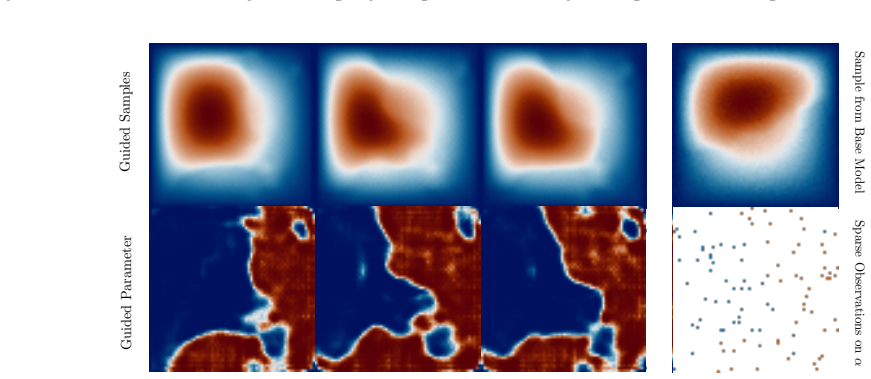
- Guidance on the recovered parameter field during sampling lets the model condition on sparse parameter observations even though the base model never saw parameters.
- Boundary conditions that contradict the training data can be imposed post hoc, with increasing $\lambda_x$ enforcing the desired boundary while the model remains close to the learned manifold.
Reading between the lines
- Because the surrogate $\alpha$-flow is constructed from the current state estimate rather than a learned base process, the theoretical tilted-distribution guarantee of Adjoint Matching should not be expected to hold exactly when $\lambda_f > 0$; the method is better understood as a regularized heuristic whose effective target is set jointly by the residual and the anchoring cost.
- The same machinery should extend to parameter-dependent constraints beyond PDE residuals, such as conservation laws, inequality constraints, or differentiable simulator residuals, whenever a weak-form or differentiable residual can be defined.
- A direct test of the tilt would compare the empirical fine-tuned distribution against the analytically tilted target on a linear-Gaussian PDE where $p_r$ is computable; such a test would clarify how much of the benefit comes from the Adjoint Matching guarantee rather than from residual regression alone.
Editorial analysis
A structured set of objections, weighed in public.
Referee Report
Summary. The paper proposes a post-training fine-tuning method for flow-matching generative models that enforces PDE constraints and infers latent parameters. The approach augments the state with a latent parameter process, defines a surrogate base flow for α via an inverse predictor φ trained to minimize weak-form PDE residuals, and applies Adjoint Matching to steer the joint process toward low-residual solutions. Experiments on Darcy flow and acoustic wave equations report reduced weak and strong residuals (Tables 1 and 3), preserved distributional statistics with regularization (Table 2), and visual demonstrations of guided sampling and boundary enforcement.
Significance. The idea of using weak-form residuals as a reward to tilt a pre-trained generative model, together with a jointly evolved latent parameter, is timely and potentially useful for scientific applications where paired parameter-solution data are unavailable. The paper has concrete strengths: the weak-residual formulation is described in detail; quantitative residual reductions in Tables 1 and 3 support the core fine-tuning claim; the distributional metrics in Table 2 address diversity preservation; and the authors promise code and dataset-generation scripts. However, the central inverse-problem claim of 'accurate recovery of latent coefficients' is not directly evaluated, and the theoretical grounding through Adjoint Matching is invoked under conditions (f=0, a valid base process) that the method's surrogate α-flow and control-dependent running cost do not satisfy. The contribution is therefore promising but currently under-supported.
major comments (3)
- [Section 4; Algorithm 1; Table 2] The paper's headline claim of 'accurate recovery of latent coefficients' is not supported by any per-sample comparison of predicted parameters against ground truth. Algorithm 1 (line 1) trains φ to minimize the same weak residual Rweak that is later used as the fine-tuning reward, and Table 2 reports only pointwise marginal statistics (MMSErel, SMSErel, Diversityrel) for α, which do not measure the error of an individual inferred coefficient field. For the Darcy problem a fixed pressure field can be consistent (at the level of the weak residual) with many different permeability fields, and the normalization by the integral of α over the test-function support in Appendix C is a practical safeguard rather than an identifiability condition. Without a per-sample ground-truth error (e.g., relative L2 error of α and c on a held-out set), the fine-tuning could lower residuals while parameters drift along the zero-residual manifold, exactly the failure mode the current protocol cannot detect.
- [Section 3, Eqs. (1)-(3)] The theoretical grounding of Adjoint Matching is invoked under conditions that the proposed joint process does not satisfy. The consistency result cited from Domingo-Enrich et al. (2025) is stated for f=0 and for a base generative process with a well-defined flow; here the surrogate base flow v^base_{t,α}=(φ(hat x_1)−α_t)/(1−t) is not an independent generative process, since hat x_1 depends on the current state x_t and φ is trained only to minimize the weak residual. Moreover, the running cost f(α)=λ_f||v^ft_{t,α}−v^reg_{t,α}||² depends on the control through v^ft_{t,α}=v^base_{t,α}+σu_α, so it is not a state-only cost as required in Eq. (1), and the lean-adjoint equation (2) omits the additional terms that a control-dependent cost would introduce. The paper acknowledges the f=0 condition for the tilt guarantee but does not analyze the f≠0 case. As written, the claim that the method 'extends Adjoint Matching' and inherits its distributional guarantees is not justified; either remove f and rely on terminal rewards only, or provide an analysis (or clearly label the procedure as a heuristic).
- [Section 4, Tables 1-3; Appendix E] The empirical evaluation provides no quantitative comparison against any competing physics-constraint method in the main text, and all quantitative results come from single training runs. Tables 1 and 3 compare the fine-tuned model only to the base FM model; the only comparison to another method (ECI, Cheng et al. 2024) appears in Appendix E and is visual, with the authors themselves noting that the comparison is 'not entirely fair.' No error bars across random seeds are given for any table, so the robustness of the reported residual reductions is unknown. At least one quantitative baseline (a projection-based sampler such as ECI or a physics-informed diffusion baseline) and mean±std over multiple seeds are needed to support the claim that the proposed fine-tuning is a competitive way to enforce PDE constraints.
minor comments (5)
- [Section 3] The terminal cost g(˜X_1) is never defined explicitly; Eq. (2) uses λ_x∇_x g and λ_α∇_α g, and the experiments tune λ_x and λ_α, but the reader cannot tell how g combines Rweak, RBC, and any observation terms. Please state the exact terminal cost used in each experiment.
- [Algorithm 1] Line 9 defines v^base_{α,t} using 'ˆαft_1', whereas the text in Section 3 defines the surrogate base flow via the base-model one-step estimate φ(hat x^base_1). Please clarify which state (base or fine-tuned) is used and correct the notation.
- [Appendix A] 'recorded every ten five steps' appears to be a typo; please specify the actual frame cadence and verify that the time range [0, 0.315] is consistent with 64 frames.
- [Throughout] Minor typos such as 'pathalogical' (Section 2), 'sparese' and 'reovered' (Appendix E), 'ressources' (Appendix C), and 'naïvely' (Section 3) should be corrected.
- [Section 4, denoising experiment] The observation noise level σ_ε in ilde{x}=x+σε is not specified; please report it in the appendix and explain how it relates to the test-function length scales.
Circularity Check
Partially self-referential evaluation: the inverse predictor φ is trained on the same weak PDE residual that later serves as the fine-tuning reward, so residual reductions do not by themselves establish accurate recovery of the true latent coefficients.
-
fitted input called prediction
[Section 3 'Joint Evolution' and Algorithm 1 (Appendix C)]
"On fully denoised samples, we can train an inverse predictor, i.e., φ(x1) = α1, such that the weak PDE residual is minimised. As a naïve approach, this already induces a joint distribution over (x1, α1) via the push-forward through φ. ... Pretrain φ based on x1 samples generated with vbase_x by minimizing Rweak(x1, φ(x1))"
The predictor φ is fitted to minimize Rweak(x1, φ(x1)) on samples from the base model, and the same weak residual is then used as the physics reward that steers fine-tuning, with the frozen φ supplying α1. Consequently, the reported residual Rweak(x1, φ(x1)) measures how well the generated state fits the zero-residual manifold selected by φ itself, not how close φ(x1) is to the true physical parameter. For Darcy flow the weak form is non-identifying for a given pressure field: many permeability fields can make the weak inner products small. Yet no per-sample comparison between predicted and ground-truth a or c is reported; Table 2 only gives pointwise mean/variance statistics.
full rationale
The paper's core residual-reduction claim has independent physical content: the weak-form residual is an external benchmark evaluated on generated fields, and fine-tuning also reduces strong residuals and boundary penalties, so the overall physics-consistency result is not merely a restatement of the training loss. However, the inverse-problem claim is partially self-referential. The latent parameter α is produced by φ, which is pre-trained to minimize Rweak, and the same Rweak is reused as the terminal reward with α supplied by φ. Residual reduction at the self-selected parameter does not certify that the predicted parameter equals the true one, especially without identifiability conditions or per-sample ground-truth parameter error. This is a fitted-input-called-prediction pattern rather than a definitional collapse, because the fine-tuning still reshapes the state distribution and the distributional statistics in Table 2 provide some external anchor against the data. The ad hoc surrogate base flow for α and the nonzero running cost also weaken the theoretical guarantee from Domingo-Enrich et al., but that is a correctness risk rather than circularity. Overall, one load-bearing evaluation loop is circular, warranting a score of 4.
Assumptions & free parameters
free parameters (7)
- lambda_x (state reward weight) =
15k for Darcy denoising; 15k-20k for misspecified boundary; not reported for acoustics
- lambda_f (parameter regularization weight) =
0.1 (main); 0.001-0.1 in ablation; 0 for pure Adjoint Matching
- lambda_alpha (adjoint terminal weight for alpha) =
not reported
- N_test (test functions per residual evaluation) =
4096 in 2D, 1000 in 3D
- test-function length-scale range [sigma_min, sigma_max] =
[3,10] for Darcy denoising; [1,20] for misspecified and acoustic experiments
- K_sub (tail refinement subdivisions) =
5 in 2D, 3 in 3D
- zeta (guidance strength) =
not reported
assumptions (6)
- domain assumption Adjoint Matching consistency result for f=0 and memoryless noise (Domingo-Enrich et al. 2025), i.e. minimizing Eq. 3 yields the tilted distribution p_r ∝ e^{-λ g} p.
- standard math Integration by parts with C_0^1 test functions justifies the weak-form residual expressions for Darcy and acoustic equations.
- domain assumption The governing equations and boundary conditions are known and correctly specified (Darcy zero Dirichlet; acoustic reflective Neumann).
- domain assumption The random Wendland-wavelet test-function family with mollifier provides a low-variance, bias-free proxy for PDE residual.
- ad hoc to paper The inverse predictor phi can be trained on base-model samples alone and yields parameter estimates meaningful enough to define surrogate flows.
- ad hoc to paper The surrogate base flow v_base_alpha = (phi(hat x_1)-alpha_t)/(1-t) behaves as a valid base generative process for Adjoint Matching.
Cite this review
Pith. "Pith review of Physics-Constrained Fine-Tuning of Flow-Matching Models for Generation and Inverse Problems." pith.science (2026). https://pith.science/paper/57VKYP4V
@misc{pith2026250809156,
  author       = {Pith},
  title        = {Pith review of: Physics-Constrained Fine-Tuning of Flow-Matching Models for Generation and Inverse Problems},
  year         = {2026},
  howpublished = {\url{https://pith.science/paper/57VKYP4V}},
  note         = {Machine review of arXiv:2508.09156}
}
read the original abstract
We present a framework for fine-tuning flow-matching generative models to enforce physical constraints and solve inverse problems in scientific systems. Starting from a model trained on low-fidelity or observational data, we apply a differentiable post-training procedure that minimizes weak-form residuals of governing partial differential equations (PDEs), promoting physical consistency and adherence to boundary conditions without distorting the underlying learned distribution. To infer unknown physical inputs, such as source terms, material parameters, or boundary data, we augment the generative process with a learnable latent parameter predictor and propose a joint optimization strategy. The resulting model produces physically valid field solutions alongside plausible estimates of hidden parameters, effectively addressing ill-posed inverse problems in a data-driven yet physicsaware manner. We validate our method on canonical PDE benchmarks, demonstrating improved satisfaction of PDE constraints and accurate recovery of latent coefficients. Our approach bridges generative modelling and scientific inference, opening new avenues for simulation-augmented discovery and data-efficient modelling of physical systems.
Figures


Figures from the paper (14 more)



Reference graph
Works this paper leans on
-
[2]
arXiv preprint arXiv:2505.12882
PhyDA: Physics-Guided Diffusion Models for Data Assimilation in Atmospheric Systems. arXiv preprint arXiv:2505.12882. Wen, G.; Li, Z.; Azizzadenesheli, K.; Anandkumar, A.; and Benson, S. M. 2022. U-FNO – An enhanced Fourier neu- ral operator-based deep-learning model for multiphase flow. arXiv:2109.03697. Xu, R.; Wang, H.; Kementzidis, G.; Si, C.; and Deng, Y
arXiv 2022
-
[3]
APOD: Adaptive PDE-Observation Diffusion for Physics-Constrained Sampling. In ICML 2025 Workshop on Assessing World Models. Zhang, H.; Li, Y .; and Huang, J. 2024. DiffusionVel: Multi- Information Integrated Velocity Inversion Using Generative Diffusion Models. arXiv:2410.21776. Zhang, L.; Rao, A.; and Agrawala, M. 2023. Adding condi- tional control to te...
arXiv 2021
-
[2025]
arXiv preprint arXiv:2506.08604
Flow Matching Meets PDEs: A Unified Frame- work for Physics-Constrained Generation. arXiv preprint arXiv:2506.08604. Bansal, A.; Chu, H.-M.; Schwarzschild, A.; Sengupta, S.; Goldblum, M.; Geiping, J.; and Goldstein, T. 2023. Univer- sal Guidance for Diffusion Models. arXiv:2302.07121. Bastek, J.-H.; Sun, W.; and Kochmann, D. 2024. Physics- Informed Diffus...
arXiv 2023
Reviewed August 6, 2026 · model on record in the stance chip above.
Discussion (0). Continue with ORCID to comment.