REVIEW 3 major objections 5 minor 3 references
Transfer Learning for Classification under Decision Rule Drift with Application to Optimal Individualized Treatment Rule Estimation
T0 review · 3 major / 5 minor · reviewed 2026-08-05 · deepseek-v4-flash
Pith's one-line read When the Bayes decision boundary shifts by a low-dimensional geometric transform, transfer learning can beat target-only classifiers.
desk verdict The core idea is genuinely new and worth referee time, but the paper's main theorem is not proven as written due to a load-bearing error in the supplementary ERM proof. read the letter →
The pith
A machine-rendered reading of the paper's core claim, the machinery that carries it, and where it could break.
The reading
What carries the argument
The load-bearing object is the decision-rule drift model (3): d_H(G_{f*_Q}, h(G_{f*_P}, θ*)) ∨ d_H(G^c_{f*_Q}, h(G_{f*_P}, θ*)^c) ≤ δ, where h is a pre-specified parametric geometric transformation such as translation or rotation, θ* is low-dimensional, and d_H is Hausdorff distance. This assumption turns the transfer problem into a p-dimensional ERM: after a source SVM estimates G_{f*_P}, the method solves a 0-1-loss calibration problem for θ on one target half, then selects among the calibrated rule, a target-only SVM, and the source rule using the other half. The Lipschitz property of h under symmetric difference gives a VC-type entropy bound of the transformed rule class, and the split-s
What would settle it
Take the proof of Theorem 4 in Supplement A.2 and substitute the correct loss difference -Y(1_A - 1_B) for g; if the resulting empirical-process bound cannot recover the exponent (1+α_Q)/(2+α_Q), the rate is unproven. A concrete check in the one-dimensional translation example with α_Q = 1, p = 1, and n_P huge: measure the excess risk against n_Q; a decay shallower than (log n_Q/n_Q)^{2/3} across repeated simulations would contradict the calibrated-transfer rate claimed in Theorem 1.
Extended reading notes
Core claim
The paper's central claim is Theorem 1: for any pair of distributions satisfying the margin, modified geometric noise, strong density, and decision-rule drift conditions, the final classifier selected by sample splitting satisfies R_Q(G_f̂_Q,final) - R*_Q = O_p( A_{n_P,n_Q} ∧ B_{n_Q} + n_Q^{-(1+α_Q)/(2+α_Q)} ) uniformly over the model class. Here A_{n_P,n_Q} is the calibrated-transfer rate containing (n_P^{-β_P+ε_P})^{α_P/(1+α_P)} for the source SVM, δ^{γ_Q} for the boundary noise, and (p log n_Q/n_Q)^{(1+α_Q)/(2+α_Q)} for the target-side calibration, while B_{n_Q} is the target-only Gaussian-SVM rate. The minimum with B prevents negative transfer. This means that when n_P is large, p is muc
Load-bearing premise
The paper's central rate depends on the calibration step in Theorem 4, but the proof of that step starts from the equality R_Q(h(G_f̂_P, θ̂)) - R_Q(h(G_f̂_P, θ*)) = E_Q[g(θ̂)] - E_{Q,n}[g(θ̂)] with g = 1_A - 1_B; for labels in {−1, 1} the true 0-1 loss difference is -Y(1_A - 1_B), so this identity fails and the displayed (p log n_Q/n_Q)^{(1+α_Q)/(2+α_Q)} rate is not actually derived in the preprint.
Editorial extensions
If this is right
- Large source, small target, and genuinely low-dimensional boundary drift: the target excess risk approaches the parametric rate (p log n_Q/n_Q)^{(1+α_Q)/(2+α_Q)}, which is faster than the Gaussian-SVM target-only rate and nearly dimension-free.
- Small boundary misspecification is tolerated: as long as the Hausdorff noise δ is small, its contribution enters only as δ^{γ_Q}, so a perfect transform is not required.
- Negative transfer is guarded by design: the final rule's risk is the minimum of the calibrated, target-only, and source-only risks up to the aggregation cost, so a failed transfer cannot do much worse than target-only SVM.
- The same calibrated transfer applies to optimal individualized treatment rules under unconfoundedness and overlap, so a large observational source can improve treatment decisions in a small target population under posterior drift.
- The framework broadens posterior-drift transfer from regression-function assumptions to purely geometric boundary assumptions, covering rotations and translations without restricting the regression functions themselves.
Reading between the lines
- Extension: a natural next step is to estimate the transformation family itself from data—for example, a dictionary of translations, rotations, and affine maps selected by the same held-out split—rather than requiring the user to pre-specify h; the paper's own validation-based suggestion points in this direction.
- Extension: because the calibrated rule replaces the fixed source-transfer cost ∥θ*∥₂ by the ERM cost (p log n_Q/n_Q)^{(1+α_Q)/(2+α_Q)}, the theorem implies that the most valuable source information is the boundary shape, not the source labels; the same calibration rationale might extend to semisupervised or covariate-shift settings.
- Extension: in the ITR application the propensity scores are taken as known in both populations; plugging in estimated propensities would add an estimation term, and the paper does not analyze that practical variant.
- Extension: the rate's dependence on the target margin parameter α_Q suggests a measurable diagnostic—if one can estimate the local mass of |2η_Q−1| near the boundary, one can predict ex ante whether transfer will beat target-only SVM.
Signed reviews
Editorial analysis
A structured set of objections, weighed in public.
Referee Report
Summary. The paper proposes a transfer learning framework for binary classification under 'decision rule drift': the Bayes decision boundary of the source distribution is assumed to be related to the target boundary through a known low-dimensional parametric transformation h(G,θ), up to a Hausdorff noise δ. The method estimates the source boundary with an SVM, calibrates the transformation parameter θ by empirical risk minimization on a portion of the target data, trains a target-only SVM, and then selects among the candidate rules on a validation split. The main theorem (Theorem 1) claims that the final classifier attains excess risk of order A_{n_P,n_Q} ∧ B_{n_Q} + n_Q^{-(1+α_Q)/(2+α_Q)} uniformly over a model class, where the calibrated-transfer component A contains (p log n_Q/n_Q)^{(1+α_Q)/(2+α_Q)}. The framework is extended to optimal individualized treatment rule estimation, and the paper reports simulations and a CPS/NSW data application.
Significance. The idea of modeling posterior drift directly through the Bayes decision boundary, rather than through regression functions, is a genuinely useful and under-explored direction. If the claimed rates were established, the method would show that a high-dimensional nonparametric classification problem can be reduced to a low-dimensional ERM problem, yielding faster rates than target-only SVM when the source sample is large and the transformation is low-dimensional. The paper also provides a clean extension to ITR estimation and a sensible negative-transfer protection mechanism via validation-based aggregation. These strengths make the paper potentially valuable. However, the central theoretical contribution currently rests on an unproven ERM calibration bound. The error is not a minor typo: it affects the main rate theorem and the advertised speed-up, so the current version does not fully support its headline claims.
major comments (3)
- [Supplementary A.2, proof of Theorem 4] The proof defines g(θ)=I{x∈h(G_fhatP,θ)}−I{x∈h(G_fhatP,θ*)} and asserts RQ(h(G_fhatP,θhat))−RQ(h(G_fhatP,θ*)) ≤ (E_Q[g(θhat)]−E_Qn[g(θhat)]). For labels in {−1,1}, the 0-1 loss difference is L_A−L_B = −Y(I_A−I_B), not I_A−I_B. The subsequent empirical-process bound, the variance calculation sup E[g^2] ≤ C1(E[g])^{α/(1+α)}, and the final rate therefore control the wrong object. E[I_A−I_B] can be small while the excess risk remains large, e.g., when the two rules make balanced errors on both sides of the Bayes boundary. Consequently the claimed rate (p log n_Q/n_Q)^{(1+α_Q)/(2+α_Q)} is not derived. Since Theorem 5 and Theorem 1 (Eq. 10) inherit this ERM component through A_{n_P,n_Q}, the advertised transfer speed-up is presently unsupported. Redefining g as Y(I_A−I_B) is a natural repair, but the margin-condition and peeling steps must then be redone; the current chain is incorrect.
- [Supplementary Lemma 4] Lemma 4 is false as stated for arbitrary f1 and f2. It asserts (R_{P,Δ}(f1)−R_{P,Δ}(f2))^{(1+α)/α} ≤ R_P(f1)−R_P(f2). A simple counterexample: let P be uniform on [0,1] with η(x)=x, take f1 to be the Bayes set {x>1/2} and f2={x<1/2}. Then R_P(f1)−R_P(f2) is negative (or can be made zero by choosing two non-Bayes rules with equal risk), while the symmetric-difference term is 1. The correct Tsybakov margin inequality bounds the distance to the Bayes rule in terms of excess risk over the Bayes risk, not the risk difference of two arbitrary classifiers. This false lemma is used in the proof of Theorem 5 in the chain leading to (R_P(G_fhatP)−R_P(G_f*_P))^{α_P/(1+α_P)}, and in Theorem 4's step d_{Q,Δ} ≤ C(E_Q[g])^{α_Q/(1+α_Q)}. This is a load-bearing issue, not a presentational one.
- [Theorem 4 and Theorem 5 proof structure] Even setting aside the sign of g, the ERM proof implicitly requires a Bernstein-type variance bound for the class h(G_fhatP,Θ) relative to its class-optimal parameter. A margin condition on Q alone does not provide such a bound when the class-optimal rule is not the Bayes rule. For two rules on opposite sides of the Bayes boundary, their risk difference can be small while their symmetric difference is large, so the variance bound d_{Q,Δ} ≤ C(E[g])^{α/(1+α)} is not generally valid. The proof needs an additional argument, e.g., absorbing the approximation error into the margin analysis or imposing a class-level margin/Bernstein condition. As written, the peeling argument does not establish the claimed ERM rate even if g is redefined to Y(I_A−I_B).
minor comments (5)
- [Supplementary Theorem 5, display after Eq. (16)] The definition of β_P in Theorem 5 contains an extra '/d' in the condition and in the second branch compared with Theorem 1 and Theorem 2. This appears to be a typographical inconsistency; please align the notation.
- [Supplementary A.2, Theorem 4 statement] The statement uses θ* in the numerator, but the proof defines θhat* as inf_{θ∈Θ}RQ(h(G_fhatP,θ)). Please clarify whether θ* denotes the population minimizer or the oracle parameter and consistently use one symbol.
- [Section 6, real data application] Algorithm 1 and Corollary 1 assume the propensity scores π_P and π_Q are known, but the CPS/NSW analysis estimates them by logistic regression. The paper should either state the additional conditions under which the theorem remains valid with estimated propensities, or explicitly present the real-data result as heuristic.
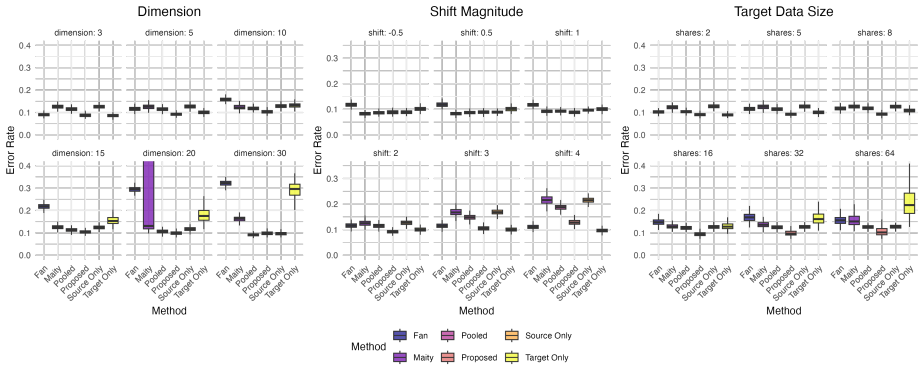
- [Figures 1–3] The simulations report means over 320 datasets but the figures do not show error bars or variability measures. Adding standard errors or boxplots would strengthen the comparisons, especially for the unstable Maity method.
- [Section 5, simulation settings] For the noisy boundary setting (b), epsilon is defined as N(0,σ²)I(x>0), which creates an asymmetry in the noise. It would be useful to state the value of σ² and justify the asymmetric specification.
Circularity Check
No circularity: the transfer parameter is estimated as an explicit ERM step, and the claimed rates follow from external SVM/empirical-process results plus explicit drift assumptions; the flagged Supplementary A.2 defect is a correctness gap, not a circular reduction.
full rationale
The derivation chain is not circular. The paper assumes a decision-rule drift model (3) with known h, unknown θ*, and Hausdorff noise δ, then estimates θ by target-data ERM (5) and bounds its excess risk using margin/geometric-noise conditions and external empirical-process/maximal-inequality tools (Mammen & Tsybakov 1999; Tsybakov 2004; Chernozhukov et al. 2014; Kitagawa & Tetenov 2018). The source SVM rate is imported from Steinwart & Scovel (2007), and the aggregation step follows Reeve et al. (2021); these are independent published results, not author-supplied assumptions. The bias terms δ^{γ_Q} and the source-risk power are derived from the explicit Hausdorff drift model, strong density, and geometric-noise assumptions, so they are consequences of the model rather than restatements of the conclusion. The only author self-citation (Zhao, Laber, Ning, Saha & Sands 2019) appears in the Discussion as a suggested future direction and is not load-bearing. One non-circular defect should be flagged separately: in Supplementary A.2, g(θ) is defined as I{x∈h(G_fhatP,θ)} − I{x∈h(G_fhatP,θ*)}, and the proof asserts RQ(h(G_fhatP,θhat))−RQ(h(G_fhatP,θ*)) ≤ E_Q[g(θhat)]−E_{Q,n}[g(θhat)]. For labels in {−1,1} the 0-1 loss difference equals −Y·(I_A−I_B), not I_A−I_B, so the displayed inequality bounds the wrong quantity and the stated (p log n_Q/n_Q)^{(1+α_Q)/(2+α_Q)} ERM rate is not derived as written. This is a substantive proof gap that affects Theorem 5 and hence the A_{n_P,n_Q} term in Theorem 1, but it is a correctness/missing-derivation issue, not a circular reduction, and therefore does not raise the circularity score.
Assumptions & free parameters
free parameters (2)
- theta* (transfer parameter) =
estimated by ERM in equation (5) on a target subset
- SVM bandwidths sigma_P, sigma_Q and regularization lambda_P, lambda_Q =
theory sets them as powers of n; experiments do not report exact tuning
assumptions (6)
- domain assumption Decision-rule drift model: there exists known h and theta* with d_H(G_Q*, h(G_P*, theta*)) and d_H(G_Q*^C, h(G_P*, theta*)^C) bounded by delta
- domain assumption h is Lipschitz under the symmetric difference measure in both theta and set arguments
- domain assumption Strong density condition with common compact support and bounded densities for P_X and Q_X
- domain assumption Margin conditions and modified geometric noise conditions hold for both P and Q
- domain assumption For ITR: SUTVA, unconfoundedness, strict overlap, bounded outcomes, and known propensity scores
- standard math Standard empirical-process inequalities and Gaussian RKHS approximation results from Steinwart and Scovel, Chernozhukov et al., and related references
Cite this review
Pith. "Pith review of Transfer Learning for Classification under Decision Rule Drift with Application to Optimal Individualized Treatment Rule Estimation." pith.science (2026). https://pith.science/paper/LVTVSPVZ
@misc{pith2026250820942,
  author       = {Pith},
  title        = {Pith review of: Transfer Learning for Classification under Decision Rule Drift with Application to Optimal Individualized Treatment Rule Estimation},
  year         = {2026},
  howpublished = {\url{https://pith.science/paper/LVTVSPVZ}},
  note         = {Machine review of arXiv:2508.20942}
}
read the original abstract
In this paper, we extend the transfer learning classification framework from regression function-based methods to decision rules. We propose a novel methodology for modeling posterior drift through Bayes decision rules. By exploiting the geometric transformation of the Bayes decision boundary, our method reformulates the problem as a low-dimensional empirical risk minimization problem. Under mild regularity conditions, we establish the consistency of our estimators and derive the risk bounds. Moreover, we illustrate the broad applicability of our method by adapting it to the estimation of optimal individualized treatment rules. Extensive simulation studies and analyses of real-world data further demonstrate both superior performance and robustness of our approach.
Figures


Figures from the paper (13 more)




Reference graph
Works this paper leans on
-
[1]
Weighted Training for Cross-Task Learning
Alexandari, A., Kundaje, A. & Shrikumar, A. (2020), Maximum likelihood with bias- corrected calibration is hard-to-beat at label shift adaptation,in ‘International Conference on Machine Learning’, PMLR, pp. 222–232. Athey, S. & Wager, S. (2021), ‘Policy learning with observational data’,Econometrica 89(1), 133–161. Audibert, J.-Y. & Tsybakov, A. B. (2007)...
work page Pith review arXiv 2020
-
[69]
57 Kitagawa, T. & Tetenov, A. (2018), ‘Who should be treated? empirical welfare maximization methods for treatment choice’,Econometrica86(2), 591–616. Kpotufe, S. & Martinet, G. (2021), ‘Marginal singularity and the benefits of labels in covariate-shift’, The Annals of Statistics49(6), 3299–3323. LaLonde, R. J. (1986), ‘Evaluating the econometric evaluati...
arXiv 2018
-
[1045]
Zhang, K., Schölkopf, B., Muandet, K. & Wang, Z. (2013), Domain adaptation under target and conditional shift,in ‘International conference on machine learning’, PMLR, pp. 819–827. Zhang, T. (2004), ‘Statistical behavior and consistency of classification methods based on convex risk minimization’,The Annals of Statistics32(1), 56–85. Zhao, B., Huang, B. & ...
work page 2013
Reviewed August 5, 2026 · model on record in the stance chip above.
Discussion (0). Continue with ORCID to comment.