Canonical Forms as Dual Volumes

Elia Mazzucchelli; Prashanth Raman

REVIEW 2 major objections 4 minor 1 cited by

Canonical Forms as Dual Volumes

T0 review · 2 major / 4 minor · reviewed 2026-08-05 · deepseek-v4-flash

Challenge this review Re-run · record.json Download PDF Read on arXiv ↗

Pith's one-line read The paper proves that many canonical forms of positive geometries are Laplace transforms of measures on dual cones, with complete monotonicity forcing hyperbolic boundaries and explicit measures for polycons and the nodal cubic.

desk verdict A useful framework linking canonical forms to Laplace transforms, with solid polycon results; the nodal cubic computation rests on an unjustified analytic continuation and several displayed formulas need repair. read the letter →

arxiv 2509.02239 v1 pith:3ZWGOSZM submitted 2025-09-02 hep-th math.AGmath.APmath.PRmath.STstat.TH

Elia Mazzucchelli , Prashanth Raman This is my paper · ORCID

classification hep-thmath.AGmath.APmath.PRmath.STstat.TH

keywords positivegeometriescanonicalformscompletemonotonicitydualvolumerepresentationshyperbolicpolynomialsspectrahedraRieszmeasurespolycons

verification ladder T0 review T1 audit T2 compute T3 formal

The pith

A machine-rendered reading of the paper's core claim, the machinery that carries it, and where it could break.

The reading

Positive geometries are regions in projective space whose volume-like information is packed into a rational function called the canonical form, defined by its poles and residues. This paper tries to show that for a substantial class of these geometries the canonical form is secretly a dual volume: it is the Laplace transform of a measure living on the convex dual of the region, and in many examples the measure is non-negative, making the canonical function completely monotone. The paper proves that complete monotonicity forces the boundary to be cut out by a hyperbolic polynomial whose hyperbolicity region is the geometry itself, and it identifies large converse families—simplex-like minimal spectrahedra and planar polycons bounded by lines and one conic—with explicit representing measures. If the picture is right, canonical-form computations can be traded for probability measures on dual cones, linking positive geometries to hyperbolicity, partial differential equations, algebraic statistics, and convex optimization.

What carries the argument

The engine is the Laplace-transform representation for completely monotone functions on a cone: on an open convex cone C, a smooth function with alternating derivatives is the Laplace transform of a unique positive measure on the dual cone C*. The paper feeds canonical forms into this via hyperbolic polynomials: if the denominator polynomial p is hyperbolic with hyperbolicity cone C, the inverse Fourier–Laplace transform of 1/p is a fundamental solution supported on C*, and differentiating it by q(∂) yields the measure for q/p. For minimal spectrahedra, p = det(A(x)) and the measure is the pushforward of the Wishart distribution along linear slices, so the Riesz kernel becomes a volume of a

What would settle it

Evaluate the claimed nodal-cubic measure (69)/(73) at a generic point of the propagation cone outside the lacuna and compare numerically with the direct inverse Fourier transform of 4/p(ξ) for the cubic (65); disagreement would show that the α→1 limit interchange fails.

Watch

Extended reading notes

Core claim

The central claim is that rational canonical forms of positive geometries are often Laplace transforms of measures on the dual cone; non-negativity of the measure defines complete monotonicity. The paper proves complete monotonicity forces the algebraic boundary to be a hyperbolic polynomial whose hyperbolicity region is the geometry (Corollary 3.17). Conversely, simplex-like minimal spectrahedral positive geometries are completely monotone, with measures built from the Wishart distribution (Corollary 3.28), and every planar polycon bounded by lines and one conic is completely monotone with an explicit arctangent measure (Theorem 4.5). For the nodal cubic, the measure is a one-fold integral

Load-bearing premise

The nodal-cubic measure is obtained by continuing the Wishart–Riesz construction from powers greater than 3/2 down to power 1, with the limit and the integration interchanged; the paper justifies this interchange only by saying the correct answer emerges, so the entire example depends on that unproven step.

Editorial extensions

If this is right

Complete monotonicity of a positive geometry forces its algebraic boundary to be a hyperbolic polynomial; any dual-volume geometry must therefore be a hyperbolicity region.
Every simplex-like minimal spectrahedral positive geometry—including the half-pizza and the nodal cubic—is completely monotone, so its canonical function is the Laplace transform of an explicit non-negative measure.
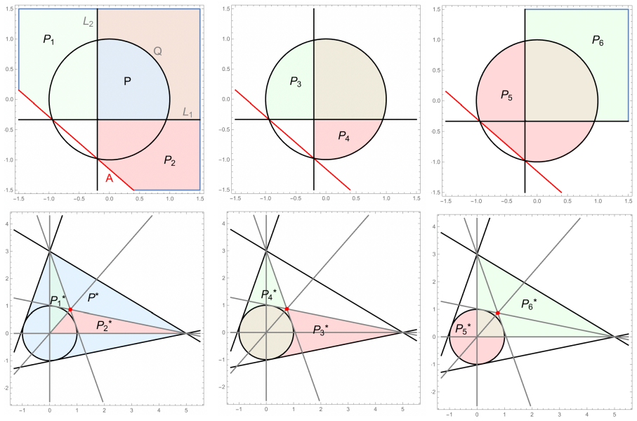
Every polycon in the projective plane bounded by lines and a single conic is completely monotone, with the measure built from arctangents of ratios of 'dual letters'.
For polycons with several conics, the measure is algorithmically computable via triangulation, and all tested examples remain non-negative.
The nodal cubic shows that measures can be transcendental—complete elliptic integrals—so even singular non-polytopal geometries fit the dual-volume picture.

Reading between the lines

Editorial extensions of the paper, not claims the author makes directly.

If the converse of Corollary 3.17 holds—every hyperbolic positive geometry is completely monotone—the entire class of hyperbolic projective geometries would admit dual volume representations, directly supporting the dual-amplituhedron program.
The 'dual letters' appearing in the measures are a dual analogue of symbol letters in scattering amplitudes; a testable extension is to check whether their vanishing loci carry the same recursive information for higher-dimensional dual geometries.
The Wishart construction suggests a tractable route beyond the paper: in non-minimal spectrahedral cones, the same fiber-integral formula could certify or falsify complete monotonicity by explicit matrix integrals.
Because a completely monotone canonical function is a moment-generating function, the paper implicitly identifies every such geometry with a rational exponential family on the dual cone; that identification could be tested statistically by sampling from the dual measure and recovering the canonical function.

Share X Bluesky LinkedIn Reddit HN

Editorial analysis

A structured set of objections, weighed in public.

Desk editor's note, referee report, and a circularity audit.

Desk Editor's Note

read the letter

Dear colleague,

I read arXiv:2509.02239. The paper does two real things. It defines completely monotone positive geometries and proves a clean structural result: a completely monotone positive geometry has hyperbolic algebraic boundary with the geometry as the hyperbolicity region (Cor 3.17). That is a nice bridge from positive geometry to the Scott–Sokal / Kozhasov–Michałek–Sturmfels circle. Cor 3.28 (simplex-like minimal spectrahedra are CM) is immediate from known Wishart results, but the observation is worth having. The polycon sections are the strongest part: Theorem 4.5, the explicit measures built from arctangents, and the triangulation algorithm are concrete and checkable. The cross-check of Example 4.11 against Wagner gives me some confidence those computations are not fantasy.

The soft spots are concentrated in the examples. The nodal cubic argument in §4.5 is the load-bearing weakness. The authors start with the Wishart density (35) for α>3/2, integrate one variable, and then take α→1. That interchange is not justified, and the stress-test note is right: for m=3, α=1 falls in the KMS case 2, where the Riesz measure is supported on rank-2 matrices and is not given by the absolutely continuous density. The sentence "justified by the fact that we obtain the correct answer" is circular. This does not kill the existence claims—Cor 3.28 already guarantees a measure—but it leaves the advertised explicit elliptic-integral formula (69)/(73) unverified. I would want either a genuine distributional computation or an independent check of the Laplace transform identity before trusting it.

There are also mechanical problems: (60) does not reduce to (59) at the cone center, and the summation limits in (52) look garbled. These are fixable, but they suggest the example sections were not carefully debugged.

Overall, this is a substantial paper that deserves a serious referee. The polycon results and the CM-hyperbolic theorem are likely correct and useful for people working on positive geometries, scattering amplitudes, or algebraic statistics. The nodal cubic example should either be fixed properly or explicitly labeled as a heuristic. Yes, send it to review, but expect heavy revision.

Best

Referee Report

2 major / 4 minor

Summary. The paper develops a dual-volume representation for canonical forms of positive geometries in projective space, expressing canonical functions as Laplace transforms of measures supported on the dual cone. It introduces the notion of a completely monotone positive geometry (Definition 3.1) and proves that such geometries must have algebraic boundary defined by a hyperbolic polynomial whose hyperbolicity region is the geometry itself (Theorem 3.16, Corollary 3.17). Using known results on hyperbolic polynomials, Riesz measures, and Wishart distributions, the authors show that simplex-like positive geometries over minimal spectrahedral cones are completely monotone (Corollary 3.28). They then compute explicit representing measures for planar geometries bounded by lines and conics, culminating in a triangulation-based proof that all such polycons are completely monotone (Theorem 4.5), and present an explicit measure for a nodal-cubic geometry in terms of an elliptic integral (Section 4.5, eq. (69)). The paper also makes conjectural connections to algebraic statistics and dual amplituhedra.

Significance. If correct, the paper gives a substantial new class of positive geometries whose canonical forms are completely monotone and admits explicit dual measures. The central structural results rest on published, externally verifiable theorems (Gårding, Atiyah–Bott–Gårding, Kozhasov–Michałek–Sturmfels, Wagner) rather than on circular reasoning, and the planar one-conic computations are detailed and partly cross-checked against Wagner's results. The proposed statistical interpretation of positive geometries is attractive and likely to stimulate further work. However, the paper's headline explicit nodal-cubic measure currently rests on an unproved analytic-continuation step, and one triangulation argument in Theorem 4.5 is not fully justified as written. These issues are load-bearing for the advertised explicit results, though they do not appear to invalidate the main structural theorems.

major comments (2)

[§4.5] The derivation of the nodal-cubic measure starts from the Wishart density (35), which is valid for α > (m−1)/2 = 1 (and is used here for α > 3/2), and then takes the limit α→1. The text justifies the interchange by saying 'the validity of commuting the limit α→1 with the integration is justified by the fact that we obtain the correct answer' (before eq. (69)). This is not an argument. For m = 3 and α = 1, Proposition 3.26, case 2 applies: the Riesz measure is supported on rank-2 psd matrices and is not given by the absolutely continuous density (35), whose exponent α − (m+1)/2 = −1 is singular. The limit of the fiber-integrated density could differ from the true α = 1 Riesz measure by contributions supported on lower-rank strata. Since the nodal-cubic measure (69)/(73) is advertised in the abstract and in the introduction as one of the paper's main explicit results, a rigorous justificat
[§4.3] The proof of Theorem 4.5 states a canonical-form triangulation Ω_P = Σ_i Ω_{P_i} with P ⊂ P_i and concludes µ_P = Σ_i µ_{P_i}. However, Proposition 4.2, which is invoked, produces signed triangulations with coefficients ε_i = ±1, and its proof for s ≥ 3 uses a subtraction. If signs are present, non-negativity of each µ_{P_i} does not imply non-negativity of the signed sum, so the claimed complete monotonicity of every polycon does not follow. If instead the P_i are intended to form a positive partition of P, the inclusion should be P_i ⊂ P, not P ⊂ P_i, and this should be stated and proved. As written, the proof of Theorem 4.5 is incomplete at a load-bearing point.

minor comments (4)

[§4.4] The text has 'Ω_P = Ω_{P1} + Ω_{P1} − Ω_{P3}'; the second term should be Ω_{P2}. Also in the proof of Proposition 4.9, 'The claim for t = 1 is precisely the content of Proposition 4.9' should refer to Proposition 4.2.
[§3.2] Equation (24) writes the representing object as µ(y) dy and calls µ a Schwartz distribution. This notation is inconsistent; a distribution need not have a density. Use dµ(y) or clarify that the absolutely continuous case is being assumed in (24).
[§4.3] Equation (60) is presented as a rewriting of (59) for r = 4, but (59) gives 2 + (1/π)Σ_{i=1}^4 arctan(...), while (60) has the form 1/2 − (1/π) arctan(...). The displayed expression does not reduce to (59) unless a nontrivial branch term k(y) is included and the constants are corrected. This should be fixed; as written it raises concerns about the reliability of the explicit formulas.
[§4.5] In eq. (69), the integral is written as ∫_{R(y)} dr dt ... . The order of integration and the domain R(y) in (70) should be stated more carefully: is the t-integral performed first, and are the limits of t dependent on r? This will be important for any numerical check.

Circularity Check

1 steps flagged · score 4.0 of 10

Nodal cubic measure in §4.5 is validated circularly: the α→1 limit interchange is justified by 'we obtain the correct answer,' i.e., by the very measure being derived.

other [Section 4.5, equation (69), page 32]
"The validity of commuting the limit α→1 with the integration is justified by the fact that we obtain the correct answer."

The Riesz measure (69)/(73) for the nodal cubic is obtained by starting from the Wishart density (35) for α>3/2, performing one integration, and taking the limit α→1. The paper acknowledges that for m=3, α=1 lies below m/2 so (35) does not directly apply. The only justification offered for the nontrivial interchange of limit and integration is that the output is 'the correct answer'—that is, the conclusion of the computation is used to validate the computation itself. No independent check (e.g., verifying the Laplace transform identity by differentiation, residue computations, or comparison with an external fundamental-solution formula for the singular cubic) is supplied. Thus the explicit nodal cubic measure is not independently derived; it is accepted because it matches the expected answ

full rationale

The paper's central classification results are largely independent of self-citation. Corollary 3.17 follows from complete monotonicity plus the holomorphic-extension argument and an external result on semialgebraic boundary components. Corollary 3.28 imports the Wishart/Riesz measure construction from Kozhasov–Michałek–Sturmfels, an external source, and the normalization constants are fixed by residue axioms rather than fitted to the target claims. Theorem 4.5 on polycons is built from explicit convolutions, triangulations, and the inverse-tangent addition formula, checked against external benchmarks such as Wagner's fundamental-solution formulas. The only significant circular step is in Section 4.5, where the α→1 limit of the Wishart density is justified by 'we obtain the correct answer.' This is a self-referential validation of the headline nodal-cubic measure: the derivation is accepted because it reproduces the expected result, without an independent proof of the limit interchange or a direct verification of the resulting Laplace representation. Because this affects an explicit computation rather than the existence theorem Corollary 3.28, the overall circularity is partial and localized, meriting a score of 4 rather than higher.

Assumptions & free parameters 3 free parameters · 9 assumptions · 3 invented entities

The framework rests on classical theorems treated as black boxes: BHWC (Theorem 2.4), Gårding/Atiyah-Bott-Gårding hyperbolic PDE theory (Theorem 3.12), and the Kozhasov-Michalek-Sturmfels determinantal/Wishart results (Proposition 3.26, from an independent group). The paper's own assumptions are modest: regularity and convexity of the positive geometry, coprimality of numerator and denominator, and two ad hoc analytic steps in the nodal cubic section (the α→1 limit and the assumed lacuna region). Free parameters are normalization constants of canonical functions fixed by residue axioms, not fitted to data.

free parameters (3)

Normalization constant 2√(1-a²) for the half-pizza canonical function (37) = 2 sqrt(1-a^2), with family parameter a in [0,1)
Chosen so the canonical form has residues ±1 along the two boundary components; fixed by the positive geometry axioms, not fitted to the claimed measure.
Normalization constant c(ℓ,q) in (44) = sqrt(-(1/2) ε_abc ε_ijk A_ai A_bj ℓ_c ℓ_k) with det(A)=1
Fixed by the requirement that residues at the two points L∩Q are ±1; a stated normalization, not a fitted constant.
Normalization constants for (46) and (66) = chosen so residues are ±1; equal to 4 for the nodal cubic
Proportionality constants fixed by the residue axioms of Definition 2.1; not inferred from the representing measure.

assumptions (9)

standard math BHWC theorem (Theorem 2.4): f is CM on an open convex cone C iff f is the Laplace transform of a positive measure on C^*.
Foundational for the dual volume representation; used throughout to identify CM with existence of the measure (Section 2.3).
standard math Gårding and Atiyah-Bott-Gårding theory of hyperbolic polynomials and fundamental solutions (Theorems 3.12, Remark 3.13).
Provides existence, support, and regularity of the Riesz measure for hyperbolic p; imported as established theory.
standard math Kozhasov-Michalek-Sturmfels [32, Cor. 4.2]: det(A(x))^{-α} is CM on its spectrahedral cone with Wishart Riesz measure.
The engine behind Corollary 3.28 and the Section 4 computations; an independent published result.
standard math Wagner's formulas for fundamental solutions of hyperbolic quartic operators in three variables [39].
Used as an external numerical cross-check in Example 4.11.
domain assumption P is a regular semialgebraic set (equal to the closure of its interior), quasi-compact and very compact (footnote 1, Section 2.1).
Needed for Corollary 3.17 to conclude P equals a hyperbolicity region, and for the cone over P to be well-defined and pointed.
domain assumption In the canonical function q/p, the polynomials p and q are coprime (Section 3, eq. (17)).
Used in the proof of Theorem 3.16 to rule out the case S_p ⊂ S_q.
domain assumption The canonical function q/p is positive on the pointed cone over P (up to sign), as required by Definition 3.1.
Positivity is part of the complete monotonicity requirement; it excludes geometries whose adjoint hypersurface meets P (cf. Lemma 3.7).
ad hoc to paper The α→1 analytic continuation of the Wishart Riesz kernel is regular and the limit commutes with the integration (Section 4.5, before eq. (69)).
Stated as a 'trick'; the paper's only justification is that 'we obtain the correct answer.'
ad hoc to paper The lacuna of the nodal cubic measure is the region L in (68), on which the measure is constant equal to 1.
Postulated following Wagner [37] and checked at one point plus numerically; not derived.

invented entities (3)

Completely monotone positive geometry (Definition 3.1)
purpose: Delimits the class of geometries whose canonical functions have positive dual volume measures.
New definition; no handle outside the property itself.
Hyperbolic positive geometry (Definition 3.18)
purpose: Positive geometry whose algebraic boundary is a hyperbolic hypersurface with hyperbolicity region P.
New definition; Corollary 3.17 shows complete monotonicity implies this property.
Dual letters f_P and g_P (Definition 4.6)
purpose: Homogeneous polynomials appearing in the arctangent argument of the measure for polycons; proposed analogues of amplitude letters.
Defined and computed within this paper; no independent measurement or externally verifiable prediction is offered beyond checkable formulas and plots.

how reviews work

0 comments

Cite this review

Pith. "Pith review of Canonical Forms as Dual Volumes." pith.science (2026). https://pith.science/paper/3ZWGOSZM

@misc{pith2026250902239,
  author       = {Pith},
  title        = {Pith review of: Canonical Forms as Dual Volumes},
  year         = {2026},
  howpublished = {\url{https://pith.science/paper/3ZWGOSZM}},
  note         = {Machine review of arXiv:2509.02239}
}

read the original abstract

We study dual volume representations of canonical forms for positive geometries in projective spaces, expressing their rational canonical functions as Laplace transforms of measures supported on the convex dual of the semialgebraic set. When the measure is non-negative, we term the geometry completely monotone, reflecting the property of its canonical function. We identify a class of positive geometries whose canonical functions admit such dual volume representations, characterized by the algebraic boundary cut out by a hyperbolic polynomial, for which the geometry is a hyperbolicity region. In particular, simplex-like minimal spectrahedra are completely monotone, with representing measures related to the Wishart distribution, capturing volumes of spectrahedra or their boundaries. We explicitly compute these measures for positive geometries in the projective plane bounded by lines and conics or by a nodal cubic, revealing periods evaluating to transcendental functions. This dual volume perspective reinterprets positive geometries by replacing logarithmic differential forms with probability measures on the dual, forging new connections to partial differential equations, hyperbolicity, convexity, positivity, algebraic statistics, and convex optimization.

Figures

Figures reproduced from arXiv: 2509.02239 by the authors.

**Figure 1.** Three positive geometries in P 2 , given in an affine chart by the shaded regions. The components of the algebraic boundary are colored in black, while the adjoint hypersurface in red. The first two examples are not positively convex, as the algebraic boundary or the adjoint hypersurface intersect the interior of the semialgebraic set. This is not the case for the last example, which is in-fact positively convex, b… view at source ↗

**Figure 2.** In green is the hyperbolicity region of ppx1, x2, x3q “ x2px 2 3 ´ x 2 2 ´ x 2 1 q on the affine slice x3 “ 1, and in black the vanishing locus of p. Pick any point in the green region. Then, any line through the point intersects V ppq in three real points, counting multiplicities. Example 3.10. The polynomial ppxq “ x2px 2 3´x 2 2´x 2 1 q is hyperbolic, as one can visually check in [PITH_FULL_IMAGE:figures/full_fi… view at source ↗

**Figure 3.** In (a), (c) and (d) we show Ppa from (36) for different values of a on the slice x3 “ 1. In (b) we show the dual Pp˚ a for a “ 1{2. equal to a 2 ´ 1, and on its roots r˘pyq in t and their relative order with respect to y3{a. We compute the discriminant of qapt, yq in t to be ∆apyq “ 4py 2 3 ´ y 2 1 ´ 2ay2y3 ` a 2 y 2 1 ` a 2 y 2 2 q. (39) We check that ∆apyq ą 0 for every y P Pp˚ a . To evaluate the integral (38) we… view at source ↗

Figures from the paper (12 more)

**Figure 4.** Figure 4: The graph of µa in (40), (41) and (42), respectively, for different values of a, and plotted on the slice C ˚Xty3 “ 1u, where C ˚ “ C is in (27). Note that for (b) and (c) the gray cuts on the vertical axis happen at locations where the measure is singular. We observe …

**Figure 5.** Figure 5: On the left, a positive geometry P inside the hyperbolicity region PpCq of a conic Q, bounded by Q and two lines L1, L2 cut out by ℓ1 “ p1, 0, 1{4q, ℓ2 “ p0, 1, 1{2q, respectively. The adjoint line of P, cut out by α, is drawn in red. In the middle, we show the dual P …

**Figure 6.** Figure 6: We show the semialgebraic sets Pi , above, and their duals P ˚ i , below, for i “ 1, . . . , 6 as in (47). These realize the canonical form triangulation (48) of the positive geometry P, appearing in blue in the first picture above with its adjoint line in red. Its du…

**Figure 7.** Figure 7: Pictorial representation of the iterative argument for building a canonical [PITH_FULL_IMAGE:figures/full_fig_p025_7.png]

**Figure 8.** Figure 8: On the left, the polycon P “ Pp1, 4q from Example 4.3 with its adjoint cubic curve in red. In the middle, its dual P ˚ , with additional curves: in blue is the vanishing locus of the degree-seven polynomial fPp, and in blue that of the degree-six gPp, see (54). On the…

**Figure 9.** Figure 9: Figure for the argument in the proof of Lemma 4.4. The sign-regions [PITH_FULL_IMAGE:figures/full_fig_p027_9.png]

**Figure 10.** Figure 10: We can then write (59) as 1 2 ´ 1 π arctan ˆ 17y 4 1´128y 3 1 y2`34y 2 1 y 2 2`128y1y 3 2`17y 4 2´2p33`20? 2qpy 2 1`y 2 2 qy 2 3`p49`40? 2qy 4 3 8 ? 2` ? 2y3p´7py 2 1`y 2 2 q`p7`4 ? 2qy 2 3 q ? y 2 3´y 2 2´y 2 1 ˙ . (60) This gives explicit expressions for the dual le…

**Figure 10.** Figure 10: On the left, an octagonal polycon Pp4, 4q as in Example 4.7 with its adjoint curve in red (which consists also of the line at infinity x3 “ 0). In the middle, its dual Pp4, 4q ˚ , with additional curves: in red is the vanishing locus of the quartic in the numerator o…

**Figure 11.** Figure 11: On the left, a curvy two-gon P, a polycon of type p2, 0, 2q, from Example 4.10. This is a positive geometry and has an adjoint curve given by the line at infinity x3 “ 0. In the middle, its dual P ˚ and on the right the plot of the measure µPp for the canonical funct…

**Figure 12.** Figure 12: The polycons Pi , above, together with their duals P ˚ i , below, see Example 4.10. These form a canonical form triangulation for the curvy two-gon in [PITH_FULL_IMAGE:figures/full_fig_p031_12.png]

**Figure 13.** Figure 13: On the left, a curvy four-gon P as in Example 4.11. This is a positive geometry with an adjoint curve given by the line at infinity x3 “ 0. In the middle, its dual and on the right a plot of the measure for its canonical function, see (64). The measure is non-negative…

**Figure 14.** Figure 14: On the left the nodal cubic cut out by (65) with its hyperbolicity region [PITH_FULL_IMAGE:figures/full_fig_p033_14.png]

Discussion (0). Continue with ORCID to comment.

Forward citations

Cited by 1 Pith paper

Reviewed papers in the Pith corpus that reference this work. Sorted by Pith novelty score. Full citation record

Global Convergence of the Return Dynamics in the Class $\mathcal{O}_C$
math.DS 2026-03 unverdicted novelty 6.0 of 10

Return dynamics on class O_C domains with fixed convex core converge globally like adaptive gradient descent of the thickness function, with fixed points equal to thickness critical points.

Reference graph

Works this paper leans on

57 extracted references · 44 canonical work pages · cited by 1 Pith paper

[1]

The Amplituhedron

Nima Arkani-Hamed and Jaroslav Trnka. “The Amplituhedron”. In: JHEP 10 (2014), p. 030. doi: 10.1007/JHEP10(2014)030. arXiv: 1312.2007 [hep-th]

arXiv 2014
[2]

Grassmannian Geometry of Scattering Amplitudes

Nima Arkani-Hamed et al. Grassmannian Geometry of Scattering Amplitudes. Cam- bridge University Press, 2016. doi: 10.1017/CBO9781316091548

doi:10.1017/cbo9781316091548 2016
[3]

Positive geometries and canonical forms

Nima Arkani-Hamed, Yuntao Bai, and Thomas Lam. “Positive geometries and canonical forms”. In: Journal of High Energy Physics 2017.11 (Nov. 2017). doi: 10 . 1007 / jhep11(2017 ) 039

work page 2017
[4]

Adjoints and Canonical Forms of Tree Amplituhedra

Kristian Ranestad, Rainer Sinn, and Simon Telen. “Adjoints and Canonical Forms of Tree Amplituhedra”. In: Math. Scand. 130 (2024), pp. 433–466. doi: 10.7146/ math.scand.a- 149816. arXiv: 2402.06527 [math.AG]

arXiv 2024
[5]

Scattering Forms and the Positive Geometry of Kine- matics, Color and the Worldsheet

Nima Arkani-Hamed et al. “Scattering Forms and the Positive Geometry of Kine- matics, Color and the Worldsheet”. In: JHEP 05 (2018), p. 096. doi: 10.1007/ JHEP05(2018 ) 096. arXiv: 1711 . 09102 [hep-th]

work page 2018
[6]

The ABJM Amplituhedron

Song He, Yu-tin Huang, and Chia-Kai Kuo. “The ABJM Amplituhedron”. In: JHEP 09 (2023). [Erratum: JHEP 04, 064 (2024)], p. 165.doi: 10.1007/JHEP09(2023)

doi:10.1007/jhep09(2023 2023
[7]

The Correlahedron

Burkhard Eden, Paul Heslop, and Lionel Mason. “The Correlahedron”. In: JHEP 09 (2017), p. 156. doi: 10.1007/JHEP09(2017)156. arXiv: 1701.00453 [hep-th]

arXiv 2017
[8]

Cosmological Polytopes and the Wavefunction of the Universe

Nima Arkani-Hamed, Paolo Benincasa, and Alexander Postnikov. “Cosmological Polytopes and the Wavefunction of the Universe”. In: (Sept. 2017). arXiv: 1709. 02813 [hep-th]

work page 2017

Show all 57 references

[9]

Stokes polytopes: the pos- itive geometry for ϕ4 interactions

Pinaki Banerjee, Alok Laddha, and Prashanth Raman. “Stokes polytopes: the pos- itive geometry for ϕ4 interactions”. In: JHEP 08 (2019), p. 067. doi: 10.1007/ JHEP08(2019 ) 067. arXiv: 1811 . 05904 [hep-th]

2019
[10]

The positive geometry for ϕp interactions

Prashanth Raman. “The positive geometry for ϕp interactions”. In: JHEP 10 (2019), p. 271. doi: 10.1007/JHEP10(2019)271. arXiv: 1906.02985 [hep-th]

2019 arXiv
[11]

On positive geometries of quartic interactions: Stokes poly- topes, lower forms on associahedra and world-sheet forms

P. B. Aneesh et al. “On positive geometries of quartic interactions: Stokes poly- topes, lower forms on associahedra and world-sheet forms”. In: JHEP 04 (2020), p. 149. doi: 10.1007/JHEP04(2020)149 . arXiv: 1911.06008 [hep-th]

2020 arXiv
[12]

On positive geometries of quartic inter- actions: one loop integrands from polytopes

Mrunmay Jagadale and Alok Laddha. “On positive geometries of quartic inter- actions: one loop integrands from polytopes”. In: JHEP 07 (2021), p. 136. doi: 10.1007/JHEP07(2021)136 . arXiv: 2007.12145 [hep-th]

2021 arXiv
[13]

Towards Positive Geometries of Massive Scalar field theories

Mrunmay Jagadale and Alok Laddha. “Towards Positive Geometries of Massive Scalar field theories”. In: (June 2022). arXiv: 2206.07979 [hep-th]

2022 arXiv
[14]

Positive Geometries of S-matrix without Color

Mrunmay Jagadale and Alok Laddha. “Positive Geometries of S-matrix without Color”. In: (Apr. 2023). arXiv: 2304 . 04571 [hep-th]. 34

2023
[15]

Cosmohedra

Nima Arkani-Hamed, Carolina Figueiredo, and Francisco Vaz˜ ao. “Cosmohedra”. In: (Dec. 2024). arXiv: 2412 . 19881 [hep-th]

2024
[16]

An invitation to positive geometries

Thomas Lam. “An invitation to positive geometries”. In: (Aug. 2022). arXiv: 2208. 05407 [math.CO]

2022
[17]

What is Positive Geom- etry?

Kristian Ranestad, Bernd Sturmfels, and Simon Telen. “What is Positive Geom- etry?” In: Le Mathematiche 80 (2025), pp. 3–16

2025
[18]

Algebraic and Positive Geometry of the Universe: from Particles to Galaxies

Claudia Fevola and Anna-Laura Sattelberger. “Algebraic and Positive Geometry of the Universe: from Particles to Galaxies”. In: arXiv preprint (2025)

2025
[19]

Eliminating spurious poles from gauge-theoretic amplitudes

Andrew Hodges. “Eliminating spurious poles from gauge-theoretic amplitudes”. In: Journal of High Energy Physics 05 (2013), p. 135

2013
[20]

Canonical forms of polytopes from adjoints

Christian Gaetz. “Canonical forms of polytopes from adjoints”. In: arXiv preprint (2025)

2025
[21]

Positivity properties of scattering ampli- tudes

Johannes Henn and Prashanth Raman. “Positivity properties of scattering ampli- tudes”. In: Journal of High Energy Physics 04 (2025), p. 150

2025
[22]

Laplace transform (PMS-6)

David Vernon Widder. “Laplace transform (PMS-6)”. In: Princeton University Press (2015)

2015
[23]

Positive geometry, local triangulations, and the dual of the Amplituhedron

Enrico Herrmann et al. “Positive geometry, local triangulations, and the dual of the Amplituhedron”. In: JHEP 01 (2021), p. 035. doi: 10.1007/JHEP01(2021)035 . arXiv: 2009 . 05607 [hep-th]

2021 doi
[24]

Towards the Amplituhedron Volume

Livia Ferro et al. “Towards the Amplituhedron Volume”. In: JHEP 03 (2016), p. 014. doi: 10.1007/JHEP03(2016)014 . arXiv: 1512.04954 [hep-th]

2016 arXiv
[25]

Positive Amplitudes In The Amplituhedron

Nima Arkani-Hamed, Andrew Hodges, and Jaroslav Trnka. “Positive Amplitudes In The Amplituhedron”. In: JHEP 08 (2015), p. 030. doi: 10.1007/JHEP08(2015)

2015 doi
[26]

Multi-loop positivity of the planar N = 4 SYM six-point amplitude

Lance J. Dixon et al. “Multi-loop positivity of the planar N = 4 SYM six-point amplitude”. In: JHEP 02 (2017), p. 112. doi: 10.1007/JHEP02(2017)112. arXiv: 1611 . 08325 [hep-th]

2017 doi
[27]

Positivity properties of five-point two-loop Wilson loops with Lagrangian insertion

Dmitry Chicherin et al. “Positivity properties of five-point two-loop Wilson loops with Lagrangian insertion”. In:JHEP 04 (2025), p. 022.doi: 10.1007/JHEP04(2025)

2025 doi
[28]

Exterior Cyclic Polytopes and Convexity of Amplituhedra

Elia Mazzucchelli and Elizabeth Pratt. “Exterior Cyclic Polytopes and Convexity of Amplituhedra”. In: (July 2025). arXiv: 2507.17620 [math.CO]

2025 arXiv
[29]

Barrier functions in interior point methods

Osman G¨ uler. “Barrier functions in interior point methods”. In: Mathematics of Operations Research 21.4 (1996), pp. 860–885

1996
[30]

8478 [hep-th]

arXiv: 1412 . 8478 [hep-th]
[31]

11456 [hep-th]

arXiv: 2410 . 11456 [hep-th]
[32]

Positivity certifi- cates via integral representations

Khazhgali Kozhasov, Mateusz Micha lek, and Bernd Sturmfels. “Positivity certifi- cates via integral representations”. In: Facets of Algebraic Geometry 2 (2019), pp. 84–114

2019
[33]

Exponential varieties

Mateusz Micha lek et al. “Exponential varieties”. In: Proceedings of the London Mathematical Society 112 (2016)

2016
[34]

Complete monotonicity for inverse powers of some combinatorially defined polynomials

Alexander D. Scott and Alan D. Sokal. “Complete monotonicity for inverse powers of some combinatorially defined polynomials”. In: Acta Mathematica 213 (2014)

2014
[35]

The analysis of linear partial differential operators

Lars H¨ ormander. The analysis of linear partial differential operators. 1. Distribution theory and Fourier analysis. Grundlehren der mathematischen Wissenschaften 256. Berlin: Springer, 1983. isbn: 3540121048

1983
[36]

An Inequality for Hyperbolic Polynomials

Lars G ˚ arding. “An Inequality for Hyperbolic Polynomials”. In: Journal of Math- ematics and Mechanics 8.6 (1959), pp. 957–965. 35

1959
[37]

Lacunas for hyperbolic differential oper- ators with constant coefficients I

M. F. Atiyah, R. Bott, and L. G ˚ arding. “Lacunas for hyperbolic differential oper- ators with constant coefficients I”. In: Acta Mathematica 124 (1970), pp. 109–189

1970
[38]

On the fundamental solutions of a class of elliptic quartic operators in dimension 3

Peter Wagner. “On the fundamental solutions of a class of elliptic quartic operators in dimension 3”. In: Journal de Math´ ematiques Pures et Appliqu´ ees81.11 (2002), pp. 1191–1206. doi: 10.1016/S0021- 7824(02)01258- 8

2002 doi
[39]

A fundamental solution of N. Zeilon’s operator

Peter Wagner. “A fundamental solution of N. Zeilon’s operator”. In: Mathemat- ica Scandinavica (2000), pp. 273–287

2000
[40]

Fundamental solutions of real homogeneous cubic operators of principal type in three dimensions

Peter Wagner. “Fundamental solutions of real homogeneous cubic operators of principal type in three dimensions”. In: (1999)

1999
[41]

Deux exemples classiques de repr´ esentation int´ egrale

Gustave Choquet. “Deux exemples classiques de repr´ esentation int´ egrale”. In:En- seignement Math´ ematique15.2 (1969), pp. 63–75

1969
[42]

On the fundamental solutions of a class of hyperbolic quartic op- erators in dimension 3

Peter Wagner. “On the fundamental solutions of a class of hyperbolic quartic op- erators in dimension 3”. In: Annali di Matematica Pura ed Applicata 184.2 (2005), pp. 139–159

2005
[43]

Positive geometries and canonical forms via mixed Hodge theory

Francis Brown and Cl´ ement Dupont. “Positive geometries and canonical forms via mixed Hodge theory”. In: arXiv preprint (2025)

2025
[44]

Linear hyperbolic partial differential equations with constant co- efficients

Lars G ˚ arding. “Linear hyperbolic partial differential equations with constant co- efficients”. In: Acta Mathematica 85 (1951), pp. 1–62

1951
[45]

Hyperbolic Polynomials and Interior Point Methods for Convex Programming

Osman G¨ uler. “Hyperbolic Polynomials and Interior Point Methods for Convex Programming”. In: Mathematical Operations Research 22 (1997)

1997
[46]

Generalized functions

Izrail’ Moiseeviˇ c Gel’fand and Georgij Evgen’eviˇ cˇSilov. Generalized functions. Vol. 2, Spaces of fundamental and generalized functions . Academic Press, 1968

1968
[47]

Adjoints and Canonical Forms of Polypols

Kathl´ en Kohn et al. Adjoints and Canonical Forms of Polypols . 2024

2024
[48]

The analysis of linear partial differential operators

Lars H¨ ormander. The analysis of linear partial differential operators. 2. Differ- ential operators with constant coefficients . Grundlehren der mathematischen Wis- senschaften 257. Berlin: Springer, 1983. isbn: 3540121390

1983
[49]

Algebraic boundaries of convex semi-algebraic sets

Rainer Sinn. “Algebraic boundaries of convex semi-algebraic sets”. In: Research in the Mathematical Sciences 2.1 (2015), p. 3

2015
[50]

Linear matrix inequality representation of sets

J William Helton and Victor Vinnikov. “Linear matrix inequality representation of sets”. In: Communications on Pure and Applied Mathematics: A Journal Issued by the Courant Institute of Mathematical Sciences 60.5 (2007), pp. 654–674

2007
[51]

The Analysis of Linear Partial Differential Operators: Distribu- tion theory and Fourier analysis

Lars H¨ ormander. The Analysis of Linear Partial Differential Operators: Distribu- tion theory and Fourier analysis . Springer-Verlag, 1983

1983
[52]

A Note on the Hyperbolicity Cone of the Specialized V´ amos Polynomial

Mario Kummer. “A Note on the Hyperbolicity Cone of the Specialized V´ amos Polynomial”. In: Acta Applicandae Mathematicae 144.1 (Dec. 2015), pp. 11–15

2015
[53]

From polygons and sym- bols to polylogarithmic functions

Claude Duhr, Herbert Gangl, and John R. Rhodes. “From polygons and sym- bols to polylogarithmic functions”. In: JHEP 10 (2012), p. 075. doi: 10.1007/ JHEP10(2012 ) 075. arXiv: 1110 . 0458 [math-ph]

2012
[54]

Hyperbolicity cones of elementary symmetric polynomials are spectrahedral

Petter Br¨ and´ en. “Hyperbolicity cones of elementary symmetric polynomials are spectrahedral”. In: Optimization Letters 8.5 (2014), pp. 1773–1782

2014
[55]

Classical Polylogarithms for Amplitudes and Wil- son Loops

Alexander B. Goncharov et al. “Classical Polylogarithms for Amplitudes and Wil- son Loops”. In: Phys. Rev. Lett. 105 (2010), p. 151605.doi: 10.1103/PhysRevLett. 105 . 151605. arXiv: 1006 . 5703 [hep-th]. 36

2010 doi
[57]

Byrd and Morris D

Paul F. Byrd and Morris D. Friedman. Handbook of elliptic integrals for engineers and physicists . Vol. 67. Springer, 2013. 37

2013
[165]

00951 [hep-th]

arXiv: 2306 . 00951 [hep-th]

Pith tools

Reviewed August 5, 2026 · model on record in the stance chip above.

[1] [1]

The Amplituhedron

Nima Arkani-Hamed and Jaroslav Trnka. “The Amplituhedron”. In: JHEP 10 (2014), p. 030. doi: 10.1007/JHEP10(2014)030. arXiv: 1312.2007 [hep-th]

arXiv 2014

[2] [2]

Grassmannian Geometry of Scattering Amplitudes

Nima Arkani-Hamed et al. Grassmannian Geometry of Scattering Amplitudes. Cam- bridge University Press, 2016. doi: 10.1017/CBO9781316091548

doi:10.1017/cbo9781316091548 2016

[3] [3]

Positive geometries and canonical forms

Nima Arkani-Hamed, Yuntao Bai, and Thomas Lam. “Positive geometries and canonical forms”. In: Journal of High Energy Physics 2017.11 (Nov. 2017). doi: 10 . 1007 / jhep11(2017 ) 039

work page 2017

[4] [4]

Adjoints and Canonical Forms of Tree Amplituhedra

Kristian Ranestad, Rainer Sinn, and Simon Telen. “Adjoints and Canonical Forms of Tree Amplituhedra”. In: Math. Scand. 130 (2024), pp. 433–466. doi: 10.7146/ math.scand.a- 149816. arXiv: 2402.06527 [math.AG]

arXiv 2024

[5] [5]

Scattering Forms and the Positive Geometry of Kine- matics, Color and the Worldsheet

Nima Arkani-Hamed et al. “Scattering Forms and the Positive Geometry of Kine- matics, Color and the Worldsheet”. In: JHEP 05 (2018), p. 096. doi: 10.1007/ JHEP05(2018 ) 096. arXiv: 1711 . 09102 [hep-th]

work page 2018

[6] [6]

The ABJM Amplituhedron

Song He, Yu-tin Huang, and Chia-Kai Kuo. “The ABJM Amplituhedron”. In: JHEP 09 (2023). [Erratum: JHEP 04, 064 (2024)], p. 165.doi: 10.1007/JHEP09(2023)

doi:10.1007/jhep09(2023 2023

[7] [7]

The Correlahedron

Burkhard Eden, Paul Heslop, and Lionel Mason. “The Correlahedron”. In: JHEP 09 (2017), p. 156. doi: 10.1007/JHEP09(2017)156. arXiv: 1701.00453 [hep-th]

arXiv 2017

[8] [8]

Cosmological Polytopes and the Wavefunction of the Universe

Nima Arkani-Hamed, Paolo Benincasa, and Alexander Postnikov. “Cosmological Polytopes and the Wavefunction of the Universe”. In: (Sept. 2017). arXiv: 1709. 02813 [hep-th]

work page 2017