REVIEW 1 major objections 8 minor 46 references
A neural network can reconstruct a quantum lattice's disorder potential from a single-energy image of the local density of states.
Reviewed by Pith at T0; open to challenge. T0 means a machine referee read the full paper against a public rubric. the ladder, T0–T4 →
T0 review · deepseek-v4-flash
2026-08-04 18:44 UTC pith:NXWOXXHH
load-bearing objection Solid empirical demonstration of LDOS-to-potential inversion; the normalization ambiguity is resolved by the appendix, and the paper deserves peer review. the 1 major comments →
Reconstructing the Hamiltonian from the local density of states using neural networks
The pith
A machine-rendered reading of the paper's core claim, the machinery that carries it, and where it could break.
Core claim
The paper's central claim is that the inverse problem—recovering the potential V(r) from a single-energy LDOS image ρ_E(r)—is practically solvable by supervised learning for a class of single-particle lattice Hamiltonians. Using an image-to-image CNN trained on normalized pairs (ρ_E, V), the authors achieve normalized mean-squared errors of 0.016 (1D, L=128) and 0.005 (2D, L=64), outperforming baseline approaches by more than an order of magnitude. The reconstruction quality degrades gracefully under noise when the network is trained with synthetic noise regularization, and remains low for disorder amplitudes V0 between 0.3 and 0.6 and correlation lengths ξ between 2 and 4.5. The authors con
What carries the argument
The key instrument is an image-to-image convolutional neural network (CNN): a convolutional network that maps one image to another image, rather than to a class label. It takes the normalized LDOS field at one energy as input and outputs the normalized disorder potential field. The network uses convolutional layers with ReLU activations and, in 2D, residual connections, with circular padding to respect periodic boundary conditions. Training data is generated by exact diagonalization of the tight-binding Hamiltonian, followed by a windowed sum of eigenstate densities, and the loss is the mean-squared error between predicted and true normalized potentials. The argument works because the LDOS i
Load-bearing premise
The load-bearing premise is that the single-particle, nearest-neighbor tight-binding model with a Gaussian random-field site potential used to generate all training data is an adequate description of the real system; if electron-electron interactions or multi-orbital physics are significant, the reconstructed 'potential' may not correspond to the physical energy landscape.
What would settle it
Apply the trained network to an LDOS image, taken from a scanning tunneling microscopy experiment on a surface whose actual potential landscape is independently known (for example, a quantum corral built by atom manipulation). If the network's predicted potential disagrees with the known landscape beyond the reported accuracy, the assumption that the simple tight-binding forward model captures the essential physics of the experiment would be falsified.
If this is right
- A single STM conductance image could be used to estimate the local potential energy landscape of a surface, enabling downstream calculations of transport and other observables.
- The low data requirement (about 1000 samples in 2D) suggests the method may be feasible when synthetic data generation is expensive, such as for interacting models.
- Noise-regularized training (injecting synthetic noise) maintains reconstruction accuracy even when test noise reaches the LDOS signal amplitude, indicating robustness to realistic experimental conditions.
- The network retains accuracy for disorder strengths and correlation lengths outside its training range (e.g., V0 ∈ [0.3,0.6], ξ ∈ [2,4.5]), implying that exact knowledge of the disorder prior may not be necessary.
- Because the model uses only a single energy slice, experiments need not perform full spectroscopic mapping to extract the Hamiltonian's potential term.
Where Pith is reading between the lines
- If validated on experimental STM data, the same image-to-image paradigm could be extended to reconstruct other spatially varying Hamiltonian parameters, such as hopping modulations or local interaction strengths, from LDOS maps at multiple energies.
- The observed failure modes—charging rings near potential minima and plateaus near maxima—suggest that incorporating physical priors (like the sign of the potential or spectral bounds) as additional loss terms could sharpen reconstruction in extreme regions.
- A multi-energy input (stacking LDOS slices at several bias voltages) could resolve ambiguities that a single slice leaves hidden, an extension the authors mention but do not test; this is a natural next experiment within their framework.
- The method's reliance on a specific forward model means its success on real materials will depend on how faithfully a tight-binding model captures the sample; surfaces with strong electron-electron correlations may require the network to be retrained on data from a more complete model.
Editorial analysis
A structured set of objections, weighed in public.
Referee Report
Summary. The paper studies the inverse problem of recovering a site-diagonal disorder potential V(r) of a single-particle nearest-neighbor tight-binding Hamiltonian (Eq. 1) from a single-energy spatial map of the LDOS (Eq. 2). The authors generate synthetic training pairs from correlated Gaussian random-field disorder in 1D and 2D, normalize both fields, and train convolutional image-to-image networks to map the normalized LDOS to the normalized potential. They report test MSE L≈0.016 (1D, L=128) and L≈4.6×10^-3 (2D, L=64), far below a linear fit and translation-augmented k-NN baselines (Table I). They also study robustness to added noise with noise-injected training and show modest out-of-distribution generalization around the training values V0=0.5, ξ=3. The paper frames the result as a step toward STM-based Hamiltonian reconstruction and explicitly limits the setting to noninteracting, single-orbital tight-binding with fixed hopping.
Significance. If the reported accuracy holds, the paper is a useful empirical demonstration that a CNN can approximate the inverse of the LDOS map within a disordered noninteracting tight-binding model, using modest data and compute (<1 GPU hour). Strengths include a clean train/validation/test split, hyperparameter tuning on validation, comparison against two baselines, honest worst-case examples, and an explicit statement of model limitations in Section IV. The appendix's global-normalization statement preserves the disorder amplitude in the target, so the reported MSE is not merely shape recovery. The paper does not overclaim uniqueness: it acknowledges that the inverse problem is ill-posed in general and frames the result as distribution-dependent approximate recovery. Within its stated scope, the contribution is solid, although it is an empirical benchmark rather than a new analytical method.
major comments (1)
- [§II, Eqs. (3)–(4), and Appendix A1] The normalization equations in the main text are ambiguous and, if read as per-sample standardization, would make the headline MSE (0.016/0.005) and the V0 out-of-distribution study misleading. Appendix A1 explicitly states that a global training-set normalization was used and that no sample-wise normalization was attempted, which resolves the substantive concern: the CNN target retains the V0 scale. However, the main text should be amended to refer to the global scheme, since as written a reader could reasonably interpret Eqs. (3)–(4) as per-sample and thereby misread the central numerical claim. This is a clarity issue in a load-bearing location, not a flaw in the implementation.
minor comments (8)
- [§III.A vs Appendix A2] The 1D sample count is inconsistent: Section III.A says 'we generated 12000 data points', while Appendix A2 says 'The total number of data points was N=15000'; the baseline paragraph also says 12000 points. Please reconcile and specify the exact split used.
- [§III.A] The text says 'We show the results of NN-1D on four test LDOS profiles in Fig. 2', but Fig. 2 shows three profiles (best, median, worst). Please correct.
- [Eq. (2), §II] The notation 'µ|E−E′|' should be 'µ(|E−E′|)' or the weighting function should be defined with explicit arguments, to avoid confusion with multiplication.
- [§II.C and Table II] The superscript n in 'ρ~_E^n' appears before noise is introduced in the main text. Clarify whether it denotes a noised LDOS or is a typo.
- [Fig. 2 caption] The caption says the LDOS input is shown '(right)' and the predicted potential is also '(right)'; one of these should be '(left)'.
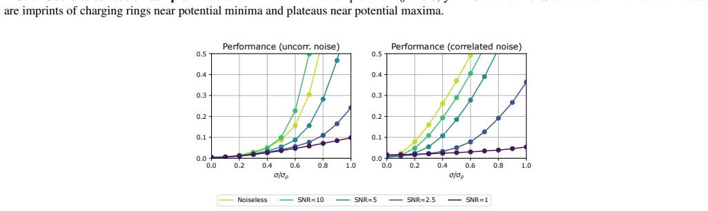
- [Appendix B] The text refers to 'Fig. 7b and Fig. 7d', but Fig. 7 appears to have two panels (uncorrelated and correlated noise). Please renumber or relabel the subfigures consistently.
- [Global reproducibility] No code, data, or random seeds are made available. Given the ML methodology, releasing the data-generation and training code would substantially improve reproducibility.
- [Fig. 5b] The out-of-distribution averages use 10 realizations per grid point but no error bars or standard errors are shown. Adding uncertainty estimates would make the claimed L≲0.1 region more persuasive.
Circularity Check
No circularity: the CNN is trained and evaluated on synthetic pairs from an independent forward model; the reported inverse mapping is a learned empirical fit, not an input-equivalent construction.
full rationale
The paper's central claim is that a CNN can approximately invert the LDOS-to-potential map of a specified tight-binding model. The forward model (Eq. 1) and LDOS definition (Eq. 2 / A1) generate synthetic training pairs; the CNN is a generic image-to-image regressor trained by MSE loss (Eqs. 5-6) and evaluated on held-out samples from the same distribution. This is standard supervised learning: the target V is not defined in terms of the input rho, and the network weights are free parameters fit to the data. The baselines (single-parameter fit, k-NN) are independent comparators and are explicitly reported as such, not presented as predictions. No step reduces a claimed result to its own input by construction. The only internal inconsistency is the normalization definition: Sec. II (Eqs. 3-4) writes per-sample mean/std, while Appendix A2 states a global training-set normalization and explicitly says 'We did not attempt sample-wise normalization.' This is a correctness/ambiguity concern, not circularity: it affects what the reported MSE measures (absolute vs. shape recovery) but does not make the CNN's output equal to its input by definition. There are no load-bearing self-citations: the only author self-citation is a contextual review reference (Ref. [22]) used to motivate STM imaging, not to justify the inverse result. The paper explicitly acknowledges limitations (single-orbital, noninteracting model) in Sec. IV, which further supports that no universal physical law is being claimed. Thus the derivation chain is self-contained and non-circular.
Axiom & Free-Parameter Ledger
free parameters (4)
- NN-1D hyperparameters =
Nc=112, NL=6, k=5, lr=1.03e-3
- NN-2D hyperparameters =
Nc=32, NB=3, k=3, lr=7.21e-4
- Global normalization statistics =
mean/std of V and rho over training set
- Problem settings (V0, xi, E, deltaE, L) =
V0=0.5, xi=3, E=-1.5 (1D)/-1.0 (2D), deltaE=0.25, L=128/64
axioms (5)
- domain assumption The system is described by a single-particle tight-binding Hamiltonian with nearest-neighbor hopping and site-diagonal potential (Eq. 1).
- domain assumption LDOS is defined as the energy-windowed sum of eigenstate densities (Eq. 2/A1).
- domain assumption Potentials are drawn from a Gaussian random field with exponential correlation (V0, xi).
- standard math CNN with circular padding preserves the periodic boundary conditions of the lattice.
- domain assumption MSE loss on globally normalized fields is a meaningful measure of reconstruction quality.
Cite this review
Pith. "Pith review of Reconstructing the Hamiltonian from the local density of states using neural networks." pith.science (2026). https://pith.science/paper/NXWOXXHH
@misc{pith2026250909604,
  author       = {Pith},
  title        = {Pith review of: Reconstructing the Hamiltonian from the local density of states using neural networks},
  year         = {2026},
  howpublished = {\url{https://pith.science/paper/NXWOXXHH}},
  note         = {Machine review of arXiv:2509.09604}
}
read the original abstract
Reconstructing a quantum system's Hamiltonian from limited yet experimentally observable information is interesting both as a practical task and from a fundamental standpoint. We pose and investigate the inverse problem of reconstructing a Hamiltonian from a spatial map of the local density of states (LDOS) near a fixed energy. We demonstrate high-quality recovery of Hamiltonians from the LDOS using supervised learning. In particular, we generate synthetic data from single-particle Hamiltonians in 1D and 2D, train convolutional neural networks, and obtain models that solve the inverse problem with remarkably high accuracy. Moreover, we are able to generalize beyond the training distribution and develop models with strong robustness to noise. Finally, we comment on possible experimental applications to scanning tunneling microscopy, where we propose that maps of the electronic local density of states might be used to reveal a sample's unknown underlying energy landscape.
Figures



Reference graph
Works this paper leans on
-
[1]
Bairey, I
E. Bairey, I. Arad, and N. H. Lindner, Learning a Local Hamil- tonian from Local Measurements, Phys. Rev. Lett.122, 020504 (2019)
2019
-
[2]
X.-L. Qi and D. Ranard, Determining a local Hamiltonian from a single eigenstate, Quantum3, 159 (2019), 1712.01850v2
Pith/arXiv arXiv 2019
-
[3]
Cao, S.-Y
C. Cao, S.-Y . Hou, N. Cao, and B. Zeng, Supervised learning in Hamiltonian reconstruction from local measurements on eigen- states, J. Phys.: Condens. Matter33, 064002 (2020)
2020
-
[4]
S.-Y . Hou, N. Cao, S. Lu, Y . Shen, Y .-T. Poon, and B. Zeng, De- termining system Hamiltonian from eigenstate measurements without correlation functions, New J. Phys.22, 083088 (2020)
2020
-
[5]
N. Cao, J. Xie, A. Zhang, S.-Y . Hou, L. Zhang, and B. Zeng, Neural Networks for Quantum Inverse Problems, arXiv 10.48550/arXiv.2005.01540 (2020), 2005.01540
work page internal anchor Pith review Pith/arXiv arXiv doi:10.48550/arxiv.2005.01540 2005
-
[6]
Gebhart, R
V . Gebhart, R. Santagati, A. A. Gentile, E. M. Gauger, D. Craig, N. Ares, L. Banchi, F. Marquardt, L. Pezz `e, and C. Bonato, Learning quantum systems, Nat. Rev. Phys.5, 141 (2023)
2023
-
[7]
Nandy, M
S. Nandy, M. Schmitt, M. Bukov, and Z. Lenarvcivc, Recon- structing effective Hamiltonians from nonequilibrium thermal and prethermal steady states, Phys. Rev. Res.6, 023160 (2024)
2024
-
[8]
C. H. Xia, M. Kaniselvan, A. N. Ziogas, M. Mladen- ovi´c, R. Mahjoub, A. Maeder, and M. Luisier, Learning the Hamiltonian Matrix of Large Atomic Systems, arXiv 10.48550/arXiv.2501.19110 (2025), 2501.19110
work page internal anchor Pith review Pith/arXiv arXiv doi:10.48550/arxiv.2501.19110 2025
-
[9]
L. P. Garc ´ıa-Pintos, K. Bharti, J. Bringewatt, H. Dehghani, A. Ehrenberg, N. Yunger Halpern, and A. V . Gorshkov, Esti- mation of Hamiltonian Parameters from Thermal States, Phys. Rev. Lett.133, 040802 (2024)
2024
-
[10]
Lantz, N
V . Lantz, N. Abiri, G. Carlsson, and M.-E. Pistol, Deep learning for inverse problems in quantum mechanics, Int. J. Quantum Chem.121, e26599 (2021)
2021
-
[11]
Zhao, S.-X
T.-L. Zhao, S.-X. Hu, and Y . Zhang, Maximum-likelihood- estimate Hamiltonian learning via efficient and robust quantum likelihood gradient, Phys. Rev. Res.5, 023136 (2023)
2023
-
[12]
Huang, Y
H.-Y . Huang, Y . Tong, D. Fang, and Y . Su, Learning Many- Body Hamiltonians with Heisenberg-Limited Scaling, Phys. Rev. Lett.130, 200403 (2023)
2023
-
[13]
W. Yu, J. Sun, Z. Han, and X. Yuan, Robust and Efficient Hamil- tonian Learning, Quantum7, 1045 (2023), 2201.00190v4
Pith/arXiv arXiv 2023
-
[14]
A. Gu, L. Cincio, and P. J. Coles, Practical Hamiltonian learning with unitary dynamics and Gibbs states, Nat. Commun.15, 1 (2024)
2024
-
[15]
J. Haah, R. Kothari, and E. Tang, Learning quantum Hamilto- nians from high-temperature Gibbs states and real-time evolu- tions, Nat. Phys.20, 1027 (2024)
2024
-
[16]
A. Dutkiewicz, T. E. O’Brien, and T. Schuster, The advantage of quantum control in many-body Hamiltonian learning, Quantum 8, 1537 (2024), 2304.07172v3
Pith/arXiv arXiv 2024
-
[17]
Binnig, H
G. Binnig, H. Rohrer, Ch. Gerber, and E. Weibel, Surface Stud- ies by Scanning Tunneling Microscopy, Phys. Rev. Lett.49, 57 (1982)
1982
-
[18]
J. Repp, G. Meyer, S. M. Stojkovi ´c, A. Gourdon, and C. Joachim, Molecules on Insulating Films: Scanning- Tunneling Microscopy Imaging of Individual Molecular Or- bitals, Phys. Rev. Lett.94, 026803 (2005)
2005
-
[19]
K. Bian, C. Gerber, A. J. Heinrich, D. J. M ¨uller, S. Scheuring, and Y . Jiang, Scanning probe microscopy, Nat. Rev. Methods Primers1, 1 (2021)
2021
-
[20]
C. J. Chen,Introduction to Scanning Tunneling Microscopy Third Edition, V ol. 69 (Oxford university press, 2021)
2021
-
[21]
J.-X. Yin, S. H. Pan, and M. Zahid Hasan, Probing topological quantum matter with scanning tunnelling microscopy, Nat. Rev. Phys.3, 249 (2021)
2021
-
[22]
K. P. Nuckolls and A. Yazdani, A microscopic perspective on moir´e materials, Nat. Rev. Mater.9, 460 (2024)
2024
-
[23]
J. B. Goetz, Y . Zhang, and M. J. Lawler, Detecting nematic or- der in STM/STS data with artificial intelligence, SciPost Phys. 8, 087 (2020)
2020
-
[24]
J. A. Sobral, S. Obernauer, S. Turkel, A. N. Pasupathy, and M. S. Scheurer, Machine learning the microscopic form of ne- matic order in twisted double-bilayer graphene, Nat. Commun. 14, 1 (2023)
2023
-
[25]
I. S. Kuijf, W. O. Tromp, T. Benschop, N. P. Ramones, M. A. Sulangi, E. P. L. van Nieuwenburg, and M. P. Allan, Self- supervised learning for denoising quasiparticle interference data, arXiv 10.48550/arXiv.2409.08891 (2024), 2409.08891
work page internal anchor Pith review Pith/arXiv arXiv doi:10.48550/arxiv.2409.08891 2024
-
[26]
Basak, M
S. Basak, M. A. Banguero, L. Burzawa, F. Simmons, P. Salev, L. Aigouy, M. M. Qazilbash, I. K. Schuller, D. N. Basov, A. Zimmers, and E. W. Carlson, Deep learning Hamiltonians from disordered image data in quantum materials, Phys. Rev. B 107, 205121 (2023)
2023
-
[27]
Automated Structure Discovery for Scanning Tunneling Microscopy
L. Kurki, N. Oinonen, and A. S. Foster, Automated Struc- ture Discovery for Scanning Tunneling Microscopy, arXiv 10.48550/arXiv.2312.08854 (2023), 2312.08854
work page internal anchor Pith review Pith/arXiv arXiv doi:10.48550/arxiv.2312.08854 2023
-
[28]
G. J. Percebois and D. Weinmann, Deep neural networks for inverse problems in mesoscopic physics: Characterization of the disorder configuration from quantum transport properties, Phys. Rev. B104, 075422 (2021)
2021
-
[29]
G. J. Percebois, A. Lacerda-Santos, B. Brun, B. Hackens, X. Waintal, and D. Weinmann, Reconstructing the potential configuration in a high-mobility semiconductor heterostructure with scanning gate microscopy, SciPost Phys.15, 242 (2023)
2023
-
[30]
Zhang, W
K. Zhang, W. Zuo, Y . Chen, D. Meng, and L. Zhang, Beyond a Gaussian denoiser: Residual learning of deep CNN for image denoising, IEEE Trans. Image Process.26, 3142 (2017)
2017
-
[31]
S. Nah, T. Hyun Kim, and K. Mu Lee, Deep multi-scale con- volutional neural network for dynamic scene deblurring, in IEEE Conference on Computer Vision and Pattern Recognition (2017) pp. 3883–3891
2017
-
[32]
P. W. Anderson, Absence of Diffusion in Certain Random Lat- tices, Phys. Rev.109, 1492 (1958)
1958
-
[33]
An, The effects of adding noise during backpropagation training on a generalization performance, Neural Comput.8, 643 (1996)
G. An, The effects of adding noise during backpropagation training on a generalization performance, Neural Comput.8, 643 (1996)
1996
-
[34]
C. M. Bishop, Training with noise is equivalent to Tikhonov regularization, Neural Comput.7, 108 (1995)
1995
-
[35]
V . Karpukhin, O. Levy, J. Eisenstein, and M. Ghazvinine- jad, Training on synthetic noise improves robustness to natural noise in machine translation, arXiv preprint arXiv:1902.01509 10.48550/arXiv.1902.01509 (2019)
-
[36]
Zhang, A
Y . Zhang, A. Mesaros, K. Fujita, S. D. Edkins, M. H. Hamidian, K. Ch’ng, H. Eisaki, S. Uchida, J. C. S. Davis, E. Khatami, and E.-A. Kim, Machine learning in electronic-quantum-matter imaging experiments, Nature570, 484 (2019)
2019
-
[37]
Choudhary, K
K. Choudhary, K. F. Garrity, C. Camp, S. V . Kalinin, R. Va- sudevan, M. Ziatdinov, and F. Tavazza, Computational scanning tunneling microscope image database, Sci. Data8, 1 (2021)
2021
-
[38]
C. Shi, M. C. Cao, S. M. Rehn, S.-H. Bae, J. Kim, M. R. Jones, D. A. Muller, and Y . Han, Uncovering material defor- mations via machine learning combined with four-dimensional scanning transmission electron microscopy, npj Comput. Mater. 7 8, 1 (2022)
2022
-
[39]
D. Wong, J. Velasco, L. Ju, J. Lee, S. Kahn, H.-Z. Tsai, C. Ger- many, T. Taniguchi, K. Watanabe, A. Zettl, F. Wang, and M. F. Crommie, Characterization and manipulation of individual de- fects in insulating hexagonal boron nitride using scanning tun- nelling microscopy, Nat. Nanotechnol.10, 949 (2015)
2015
-
[40]
Binnig, H
G. Binnig, H. Rohrer, C. Gerber, and E. Weibel, 7 × 7 recon- struction on si(111) resolved in real space, Phys. Rev. Lett.50, 120 (1983)
1983
-
[41]
Perdereau, J
J. Perdereau, J. P. Biberian, and G. E. Rhead, Adsorption and surface alloying of lead monolayers on (111) and (110) faces of gold, J. Phys. F: Met. Phys.4, 798 (1974)
1974
-
[42]
P. Li and F. Ding, Origin of the herringbone reconstruction of Au(111) surface at the atomic scale, Sci. Adv.8, 10.1126/sci- adv.abq2900 (2022). Appendix A: Data generation, ML implementation, and baselines Numerical experiments were implemented in PyTorch 2.0 and conducted on an Nvidia A100 GPU (neural networks) or CPU (baselines). We trained image-to-im...
doi:10.1126/sci- 2022
-
[43]
Synthetic data generation We generatedNsynthetic data points with a 2/3−1/6−1/6 train-validation-test split. To produce the random potentials V(r)discussed in the main text, we generate a Gaussian random field in both one and two dimensions by first creating white noise in reciprocal space and then multiplying by p psd(k), where the power spectral density...
-
[44]
The network takes 1D input signals of lengthLand applies a sequence of 1D convolutions with circular padding to preserve periodicity using the standard PyTorch moduleConv1d
Neural networks NN-1DFor NN-1D, we employed a 1D CNN consisting ofN L hidden layers with constant channel width. The network takes 1D input signals of lengthLand applies a sequence of 1D convolutions with circular padding to preserve periodicity using the standard PyTorch moduleConv1d. Each hidden layer containsN c channels, with kernel sizekapplied acros...
-
[45]
The single-parameter linear fit was the first baseline
Baselines We compared our neural network approach against two baseline methods for the inverse mapping from normalized local density of states ˜ρE (r)to normalized disorder potential ˜V(r). The single-parameter linear fit was the first baseline. It assumes a direct proportionality between (mean-subtracted) LDOS and potential: ˜V pred(r) =α˜ρE (r)whereαis ...
-
[46]
learnability
Figure 3 and out-of-distribution study For Fig. 3c-d, we performed a “learnability” study of the 1D Anderson model. We chose system sizeL=64, correlation lengthξ=3, and disorder amplitudesV 0/t∈[0.05,1.0]. For each disorder amplitudeV 0, we generated 500 random disorder realizations, diagonalized each Hamiltonian, and stored results for reuse across diffe...
discussion (0)
Sign in with ORCID, Apple, or X to comment. Anyone can read and Pith papers without signing in.