REVIEW 1 major objections 7 minor 116 references
Astroclimes -- measuring the abundance of CO$_2$ and CH$_4$ in the Earth's atmosphere using astronomical observations
T0 review · 1 major / 7 minor · reviewed 2026-08-15 · deepseek-v4-flash
Pith's one-line read Astroclimes shows that ground-based astronomical spectra of telluric standard stars can recover the long-term rise of atmospheric CO2 and CH4.
desk verdict A well-built feasibility study for a genuinely new way to get nighttime greenhouse-gas columns from archival telluric spectra, but the profile-shape scaling and CAMS-based shift keep the CO2/CH4 numbers from being trusted yet. read the letter →
The pith
A machine-rendered reading of the paper's core claim, the machinery that carries it, and where it could break.
The reading
What carries the argument
The central object is the synthetic telluric transmission spectrum, computed from molecular cross-sections (a newly calculated low-temperature grid based on HITRAN), an atmospheric profile of pressure, temperature, and molecular abundances, and the Beer-Lambert law with additional terms for Rayleigh scattering, aerosol extinction, and collision-induced absorption by O2. The free parameters are the ground-level abundances of CO2, CH4, H2O, and O2; each molecular abundance profile from the GGG2020 pipeline is multiplied by a single scaling factor. The model is compared to observations through a cross-correlation-based log-likelihood, and the parameters are estimated with an MCMC using the emcee sampler. Column-averaged dry mole fractions are derived by integrating the retrieved number-density profiles relative to O2, whose atmospheric fraction is assumed constant.
What would settle it
A direct test would be to generate synthetic telluric spectra with the ESO Sky Model but with deliberately altered CO2 and CH4 vertical profile shapes (same ground value, different distribution with height), run the Astroclimes retrieval on them, and check whether the retrieved column-averaged dry mole fractions recover the known inputs or instead show a shape-dependent bias. Independently, comparing Astroclimes column-averaged retrievals to collocated aircraft flask profiles or TCCON measurements over the same nights at a site such as Calar Alto would reveal whether profile-shape errors produce the observed vertical offset and missing seasonal cycle.
Extended reading notes
Core claim
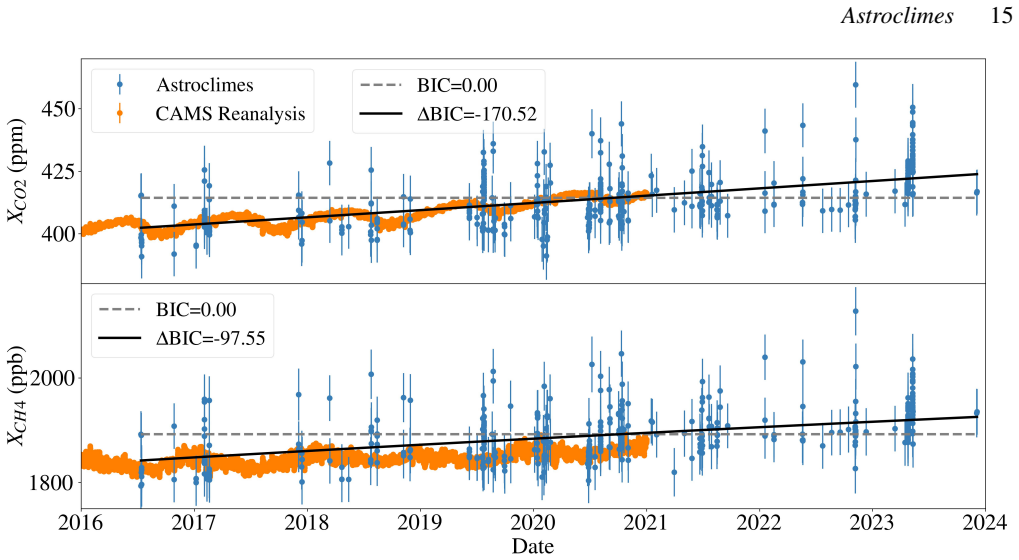
The paper's central claim is that astronomical observations of telluric standard stars, which are routinely taken for calibration and contain strong telluric absorption lines, can be used to estimate the column-averaged and ground-level dry mole fractions of CO2 and CH4 in Earth's atmosphere. Using a Markov-Chain Monte Carlo fit of synthetic transmission spectra to CARMENES near-infrared data, the authors recover the long-term upward trend of both gases over 2016 to 2023, though the seasonal cycle is not detected at a statistically significant level. The paper also quantifies the current precision limits: on hourly timescales the scatter is comparable to the individual measurement uncertainties, indicating that the residual long-term scatter is dominated by systematic effects rather than random noise.
Load-bearing premise
The retrieval assumes the vertical shape of each molecular abundance profile from the GGG2020 pipeline is correct and only scales that entire profile by a single constant; if the true shape differs, for example because the underlying flask records are extrapolated through an El Niño year, the column-averaged values will be biased even when the ground-level value fits well.
Editorial extensions
If this is right
- Archival telluric standard star spectra from high-resolution spectrographs at multiple observatories could become a new data source for nighttime greenhouse-gas column monitoring.
- The short-timescale scatter (about ±1 ppm for CO2 and ±10 ppb for CH4 within a night) suggests that once systematic offsets are understood, the method could approach the precision needed to detect regional carbon-cycle signals.
- The inability to recover seasonal cycles with the current dataset indicates that longer time baselines or better control of systematic biases are required before the method can be used for trend attribution studies.
- Applying the same algorithm to other near-infrared instruments, especially those covering the stronger O2 A-band in the visible, could improve the column-averaged retrievals and reduce scatter.
- The overall vertical shift of the retrieved abundances relative to the CAMS reanalysis points to a correctable bias that, if removed, would make the method directly comparable to established column networks.
Reading between the lines
- If the nightly precision holds after correcting the systematic offset, the method could turn existing exoplanet-atmosphere telluric calibration data into a climate dataset spanning years, enabling retrospective studies of how CO2 and CH4 columns evolved at dozens of observatory sites.
- The assumed constancy of the vertical profile shape is likely the main source of the seasonal-cycle failure; a retrieval that fits profile shape parameters (e.g., a scale height or a stratification parameter) rather than a single ground-level scaling factor might recover the seasonal signal.
- Combining the near-infrared CO2 and CH4 lines with the visible O2 A-band in a joint retrieval would anchor the dry-air column directly from the same stellar spectrum, reducing the reliance on external O2 assumptions and potentially lowering the column-averaged scatter.
- A direct test of the method's sensitivity to profile shape could be made by applying Astroclimes to spectra taken during a known El Niño event, when the extrapolated MLO and SMO flask records are most likely to be in error.
Signed reviews
Editorial analysis
A structured set of objections, weighed in public.
Referee Report
Summary. The paper presents Astroclimes, a synthetic telluric transmission code that generates model spectra from atmospheric profiles and molecular cross-sections, then fits them to high-resolution near-infrared spectra of telluric standard stars using an MCMC likelihood. The method retrieves ground-level and column-averaged dry mole fractions of CO2, CH4, H2O, and O2. The authors apply it to 436 CARMENES observations from 2016 to 2023, using GGG2020 prior profiles scaled by a single ground-level factor per molecule. Benchmarking against the CAMS EGG4 reanalysis, they report long-term scatter of ±5 ppm (ground CO2), ±9 ppm (column CO2), ±31 ppb (ground CH4), and ±42 ppb (column CH4), plus vertical offsets that they correct using the same CAMS comparison. The paper claims recovery of the long-term CO2 and CH4 trends but not their seasonal cycles, and demonstrates short-timescale scatter of order ±1 ppm and ±10 ppb that is comparable to individual MCMC uncertainties.
Significance. If the central claim holds, the method would turn routine telluric-standard observations into a nighttime greenhouse-gas column measurement capability, reusing archival data from multiple observatories. The paper has clear strengths: it uses a large, real dataset; includes a dedicated weather-balloon profile; makes honest and explicit statements about known limitations (e.g., unpropagated GGG2020 extrapolation errors in Section 3.2.4); and provides a SKYCALC benchmark for H2O that quantitatively tests the retrieval of precipitable water vapour. However, the CO2 and CH4 channels are not validated against synthetic spectra or an independent reference free of circularity, and the recovered long-term trend may be inherited from the smooth extrapolation of the GGG2020 priors. These gaps are load-bearing for the paper's main claim, so the contribution is currently more a promising proof-of-concept than a demonstrated measurement technique.
major comments (1)
- [§4, §3.2.4, Eq. (22)] The retrieval in §4 fits only a single ground-level scaling factor that multiplies the full GGG2020 prior profile; if the prior vertical shape is inaccurate, both the fitted ground-level value and the column-averaged DMF from Eq. (22) are biased in a way that a single scale factor cannot correct. Section 3.2.4 acknowledges this directly, stating that the MLO/SMO flask records are extrapolated after 2018, that El Niño conditions can corrupt the profile shape, and that the estimated extrapolation errors (0.25% for CO2, 0.6% for CH4) are not propagated into the reported uncertainties. Since the CARMENES sample spans 2016–2023, roughly half of the data use extrapolated profiles, and the extrapolation functions (19)–(20) are smooth baselines plus a fixed average seasonal cycle. The recovered long-term trend could therefore be an artifact of the smooth extrapolation in the GGG2020 priors rather than a genuine atmospheric signal. The paper provides no sensitivity test that varies the CO2 or CH4 profile shape; Section 4.2 compares only different H2O profile sources. Such a test is necessary before the trend recovery can be attributed to the measurement.
minor comments (7)
- [§3.1] The data cut from 600 to 511 observations uses an O2 range of 209500±10000 ppm; the threshold is not clearly justified, and since O2 is itself a fitted parameter, the selection could bias the final sample.
- [§3.1.2] The statement that the normalisation parameters 'did not prove to significantly alter the results' is not accompanied by a quantitative check; a brief sensitivity table would support this claim.
- [§3.2.4] The sentence reporting the extrapolation errors (0.25% for CO2, 0.6% for CH4) immediately notes that these errors are not propagated; the paper would benefit from a propagation or at least a sensitivity range in the reported uncertainties.
- [Abstract] There are several typographical issues in the abstract, such as 'Astroclimescan' and 'therently'; these should be corrected throughout the manuscript.
- [Figures 6–9] The BIC comparisons in the figure captions are hard to parse; BIC is a relative measure, so a horizontal line 'centred on 0' is an unusual baseline and the caption should state the two competing models explicitly.
- [Eq. (6)] The Rayleigh scattering expression mixes a wavelength in micrometres with an exponent involving λ; please specify the units of λ in this equation.
- [§3.3] Using the 800 hPa pressure level for surface pressures of 770–790 hPa introduces a small systematic; please state the approximate magnitude of this effect.
Circularity Check
One minor self-referential step in the CAMS vertical-offset validation; the core retrieval is otherwise self-contained.
-
other
[Section 4.3, CAMS comparison and vertical shift; Figures 10 and 11 captions]
"Therefore, when comparing our results with the CAMS reanalysis data, we apply a shift to our retrieved values based on c0 values obtained in the long-term trend fitting function. ... the Astroclimes values have been vertically shifted to match the CAMS data based on the c0 values obtained in the long-term trend fitting function described in the text."
The vertical offset added to Astroclimes before the CAMS comparison is computed from the same Astroclimes-versus-CAMS long-term trend fit, so the post-shift comparison cannot independently validate the absolute abundance level. The comparison remains informative for the long-term trend slope and for scatter, because a constant shift does not change the shape of the series or the BIC comparison, but it is circular to present the shifted match as benchmark confirmation of the offset itself. This is a validation-level circularity, not a by-construction reduction of the central retrieval.
full rationale
The central retrieval chain is self-contained: Astroclimes builds model telluric spectra from HITRAN cross-sections, atmospheric profiles, and a Beer-Lambert radiative transfer model, then fits the observed CARMENES spectra via an MCMC likelihood, retrieving ground-level abundance scaling factors and deriving column-averaged DMFs from the scaled profiles. No equation in this chain is defined in terms of the final abundance values, and the paper does not rename a known empirical pattern as a new prediction. The SKYCALC benchmark is an independent external check: Astroclimes reproduces the reported PWV values from model spectra before any comparison with CAMS. The GGG2020 profile-shape scaling is a genuine assumption and a correctness risk, but the paper explicitly acknowledges the extrapolation error and does not claim to constrain profile shape; a single scaling factor does not make the fitted trend equal to the prior trend by construction. Self-citations to Gandhi & Madhusudhan and Brogi & Line are methodological and not load-bearing circularity. The only notable circular element is the vertical-shift correction: the offset applied before the CAMS comparison is derived from the same CAMS-referenced trend fit, so the absolute-level agreement is not an independent validation. Because the long-term trend and scatter claims are shape-based and unaffected by a constant shift, the overall circularity is minor, giving a score of 2.
Assumptions & free parameters
free parameters (6)
- CO2 ground-level abundance scaling factor =
Posterior median per observation (not tabulated)
- CH4 ground-level abundance scaling factor =
Posterior median per observation (not tabulated)
- H2O ground-level abundance scaling factor =
Posterior median per observation (not tabulated)
- O2 ground-level abundance scaling factor =
Posterior median per observation (not tabulated)
- Vertical shift for CO2 =
14 ppm (ground), 15 ppm (column)
- Vertical shift for CH4 =
42 ppb (ground), 7 ppb (column)
assumptions (6)
- domain assumption HITRAN line lists and the computed cross-section grid are accurate for Earth's atmosphere.
- ad hoc to paper The vertical shape of each molecular abundance profile is known from GGG2020 and only its amplitude is free.
- domain assumption Telluric standard stars have negligible spectral features after normalization.
- domain assumption CAMS EGG4 reanalysis is an adequate reference for retrieved abundances.
- domain assumption The ESO Sky Model correctly predicts the positions of telluric emission lines.
- standard math The Beer-Lambert law and the adopted Rayleigh, aerosol and CIA parameterizations describe NIR telluric absorption.
Cite this review
Pith. "Pith review of Astroclimes -- measuring the abundance of CO$_2$ and CH$_4$ in the Earth's atmosphere using astronomical observations." pith.science (2026). https://pith.science/paper/PCEWT7RM
@misc{pith2026250910258,
  author       = {Pith},
  title        = {Pith review of: Astroclimes -- measuring the abundance of CO$_2$ and CH$_4$ in the Earth's atmosphere using astronomical observations},
  year         = {2026},
  howpublished = {\url{https://pith.science/paper/PCEWT7RM}},
  note         = {Machine review of arXiv:2509.10258}
}
abstract
Monitoring the abundance of greenhouse gases (GHGs) such as carbon dioxide (CO$_2$) and methane (CH$_4$) is necessary to quantify their impact on global warming and climate change. Although a number of satellites and ground-based networks measure the total column volume mixing ratio (VMR) of these gases, they rely on sunlight, and column measurements at night are comparatively scarce. We present a new algorithm, Astroclimes, that hopes to complement and extend nighttime CO$_2$ and CH4 column measurements. Astroclimes can measure the abundance of GHGs on Earth by generating a model telluric transmission spectra and fitting it to the spectra of telluric standard stars in the near-infrared taken by ground-based telescopes. A Markov Chain Monte Carlo (MCMC) analysis on an extensive dataset from the CARMENES spectrograph showed that Astroclimes was able to recover the long term trend known to be present in the molecular abundances of both CO$_2$ and CH$_4$, but not their seasonal cycles. Using the Copernicus Atmosphere Monitoring Service (CAMS) global greenhouse gas reanalysis model (EGG4) as a benchmark, we identified an overall vertical shift in our data and quantified the long term scatter in our retrievals. The scatter on a 1 hour timescale, however, is much lower, and is on par with the uncertainties on individual measurements. Although currently the precision of the method is not in line with state of the art techniques using dedicated instrumentation, it shows promise for further development.
Figures


Figures from the paper (8 more)



Reference graph
Works this paper leans on
-
[1]
Agust\' -Panareda A., et al., 2023, @doi [Atmospheric Chemistry and Physics] 10.5194/acp-23-3829-2023 , 23, 3829
-
[2]
Agust\' -Panareda A., et al., 2024, CAMS global greenhouse gas reanalysis (EGG4), https://ads.atmosphere.copernicus.eu/datasets/cams-global-ghg-reanalysis-egg4
2024
-
[3]
E., et al., 2014, @doi [Atmospheric Measurement Techniques] 10.5194/amt-7-647-2014 , 7, 647
Andrews A. E., et al., 2014, @doi [Atmospheric Measurement Techniques] 10.5194/amt-7-647-2014 , 7, 647
-
[4]
Artigau \'E ., et al., 2014, in Ramsay S. K., McLean I. S., Takami H., eds, Society of Photo-Optical Instrumentation Engineers (SPIE) Conference Series Vol. 9147, Ground-based and Airborne Instrumentation for Astronomy V. p. 914715 ( @eprint arXiv 1406.6992 ), @doi 10.1117/12.2055663
arXiv 2014
-
[5]
Artigau \'E ., et al., 2024, in Bryant J. J., Motohara K., Vernet J. R. D., eds, Society of Photo-Optical Instrumentation Engineers (SPIE) Conference Series Vol. 13096, Ground-based and Airborne Instrumentation for Astronomy X. p. 130960C, @doi 10.1117/12.3018994
-
[6]
Bacastow R. B., Adams J. A., Keeling C. D., Moss D. J., Whorf T. P., Wong C. S., 1980, @doi [Science] 10.1126/science.210.4465.66 , 210, 66
-
[7]
Bacastow R. B., Keeling C. D., Whorf T. P., 1985, @doi [ ] 10.1029/JD090iD06p10529 , https://ui.adsabs.harvard.edu/abs/1985JGR....9010529B 90, 10,529
-
[8]
Bailey J., Simpson A., Crisp D., 2007, @doi [ ] 10.1086/512824 , https://ui.adsabs.harvard.edu/abs/2007PASP..119..228B 119, 228
Show all 116 references
-
[9]
S., Tans P
Bakwin P. S., Tans P. P., Hurst D. F., Zhao C., 1998, @doi [Tellus B: Chemical and Physical Meteorology] 10.3402/tellusb.v50i5.16216 , 50, 401
1998 doi
-
[10]
P., Alden C
Ballantyne A. P., Alden C. B., Miller J. B., Tans P. P., White J. W. C., 2012, @doi [ ] 10.1038/nature11299 , https://ui.adsabs.harvard.edu/abs/2012Natur.488...70B 488, 70
2012 doi
-
[11]
R., Pollock H
Basilio R. R., Pollock H. R., Hunyadi-Lay S. L., 2014, in Meynart R., Neeck S. P., Shimoda H., eds, Society of Photo-Optical Instrumentation Engineers (SPIE) Conference Series Vol. 9241, Sensors, Systems, and Next-Generation Satellites XVIII. p. 924105, @doi 10.1117/12.2074164
2014 doi
-
[12]
L., Battle M., Keeling R
Bender M. L., Battle M., Keeling R. F., 1998, @doi [Annual Review of Environment and Resources] https://doi.org/10.1146/annurev.energy.23.1.207 , 23, 207
1998 doi
-
[13]
Berden G., Peeters R., Meijer G., 2000, @doi [International Reviews in Physical Chemistry] 10.1080/014423500750040627 , 19, 565
2000 doi
-
[14]
L., Lallement R., Ferron S., Boonne C., Bodichon R., 2014, @doi [ ] 10.1051/0004-6361/201322383 , https://ui.adsabs.harvard.edu/abs/2014A&A...564A..46B 564, A46
Bertaux J. L., Lallement R., Ferron S., Boonne C., Bodichon R., 2014, @doi [ ] 10.1051/0004-6361/201322383 , https://ui.adsabs.harvard.edu/abs/2014A&A...564A..46B 564, A46
2014 doi
-
[15]
A., Jones C
Betts R. A., Jones C. D., Knight J. R., Keeling R. F., Kennedy J. J., 2016, Nature Climate Change, 6, 806
2016
-
[16]
Bouchy F., et al., 2017, @doi [The Messenger] 10.18727/0722-6691/5034 , https://ui.adsabs.harvard.edu/abs/2017Msngr.169...21B 169, 21
2017 doi
-
[17]
R., 2019, @doi [ ] 10.3847/1538-3881/aaffd3 , https://ui.adsabs.harvard.edu/abs/2019AJ....157..114B 157, 114
Brogi M., Line M. R., 2019, @doi [ ] 10.3847/1538-3881/aaffd3 , https://ui.adsabs.harvard.edu/abs/2019AJ....157..114B 157, 114
2019 doi
-
[18]
Brogi M., Snellen I. A. G., de Kok R. J., Albrecht S., Birkby J., de Mooij E. J. W., 2012, @doi [ ] 10.1038/nature11161 , https://ui.adsabs.harvard.edu/abs/2012Natur.486..502B 486, 502
2012 doi
-
[19]
Brogi M., Snellen I. A. G., de Kok R. J., Albrecht S., Birkby J. L., de Mooij E. J. W., 2013, @doi [ ] 10.1088/0004-637X/767/1/27 , https://ui.adsabs.harvard.edu/abs/2013ApJ...767...27B 767, 27
2013 doi
-
[20]
J., Birkby J
Brogi M., de Kok R. J., Birkby J. L., Schwarz H., Snellen I. A. G., 2014, @doi [ ] 10.1051/0004-6361/201423537 , https://ui.adsabs.harvard.edu/abs/2014A&A...565A.124B 565, A124
2014 doi
-
[21]
Bruhwiler L., et al., 2021, @doi [Climatic Change] 10.1007/s10584-021-03001-7 , https://ui.adsabs.harvard.edu/abs/2021ClCh..165...12B 165, 12
2021 doi
-
[22]
Chatterjee A., et al., 2017, @doi [Science] 10.1126/science.aam5776 , 358, eaam5776
2017 doi
-
[23]
A., Shephard M
Clough S. A., Shephard M. W., Mlawer E. J., Delamere J. S., Iacono M. J., Cady-Pereira K., Boukabara S., Brown P. D., 2005, @doi [ ] 10.1016/j.jqsrt.2004.05.058 , https://ui.adsabs.harvard.edu/abs/2005JQSRT..91..233C 91, 233
2005 doi
-
[24]
J., Tans P
Conway T. J., Tans P. P., Waterman L. S., Thoning K. W., Kitzis D. R., Masarie K. A., Zhang N., 1994, @doi [Journal of Geophysical Research: Atmospheres] https://doi.org/10.1029/94JD01951 , 99, 22831
1994 doi
-
[25]
Cook J., et al., 2016, @doi [Environmental Research Letters] 10.1088/1748-9326/11/4/048002 , https://ui.adsabs.harvard.edu/abs/2016ERL....11d8002C 11, 048002
2016 doi
-
[26]
V., Bailey J., Kedziora-Chudczer L., 2014, @doi [ ] 10.1093/mnras/stt2465 , https://ui.adsabs.harvard.edu/abs/2014MNRAS.439..387C 439, 387
Cotton D. V., Bailey J., Kedziora-Chudczer L., 2014, @doi [ ] 10.1093/mnras/stt2465 , https://ui.adsabs.harvard.edu/abs/2014MNRAS.439..387C 439, 387
2014 doi
-
[27]
M., Betts R
Cox P. M., Betts R. A., Jones C. D., Spall S. A., Totterdell I. J., 2000, @doi [ ] 10.1038/35041539 , https://ui.adsabs.harvard.edu/abs/2000Natur.408..184C 408, 184
2000 doi
-
[28]
J., Xiong X
Crisp D., 2015, in Butler J. J., Xiong X. J., Gu X., eds, Society of Photo-Optical Instrumentation Engineers (SPIE) Conference Series Vol. 9607, Earth Observing Systems XX. SPIE, p. 960702, @doi 10.1117/12.2187291 , https://doi.org/10.1117/12.2187291
2015 doi
-
[29]
Crisp D., et al., 2017, @doi [Atmospheric Measurement Techniques] 10.5194/amt-10-59-2017 , 10, 59
2017 doi
-
[30]
Crisp D., et al., 2020, Orbiting Carbon Observatory-2 & 3 (OCO-2 & OCO-3) Level 2 Full Physics Retrieval Algorithm Theoretical Basis
2020
-
[31]
Crossfield I. J. M., 2015, @doi [Publications of the Astronomical Society of the Pacific] 10.1086/683115 , 127, 941
2015 doi
-
[32]
C., Parrish D
Derber J. C., Parrish D. F., Lord S. J., 1991, @doi [Weather and Forecasting] 10.1175/1520-0434(1991)006<0538:TNGOAS>2.0.CO;2 , 6, 538
1991 doi
-
[33]
J., et al., 2023, @doi [ ] 10.1051/0004-6361/202245217 , https://ui.adsabs.harvard.edu/abs/2023A&A...671A..24D 671, A24
Dorn R. J., et al., 2023, @doi [ ] 10.1051/0004-6361/202245217 , https://ui.adsabs.harvard.edu/abs/2023A&A...671A..24D 671, A24
2023 doi
-
[34]
E., O'Dell C
Eldering A., Taylor T. E., O'Dell C. W., Pavlick R., 2019, @doi [Atmospheric Measurement Techniques] 10.5194/amt-12-2341-2019 , 12, 2341
2019 doi
-
[35]
Fischer H., et al., 2008, @doi [Atmospheric Chemistry & Physics] 10.5194/acp-8-2151-2008 , https://ui.adsabs.harvard.edu/abs/2008ACP.....8.2151F 8, 2151
2008 doi
-
[36]
K., McLean I
Follert R., et al., 2014, in Ramsay S. K., McLean I. S., Takami H., eds, Society of Photo-Optical Instrumentation Engineers (SPIE) Conference Series Vol. 9147, Ground-based and Airborne Instrumentation for Astronomy V. p. 914719, @doi 10.1117/12.2054197
2014 doi
-
[37]
W., Lang D., Goodman J., 2013, @doi [ ] 10.1086/670067 , https://ui.adsabs.harvard.edu/abs/2013PASP..125..306F 125, 306
Foreman-Mackey D., Hogg D. W., Lang D., Goodman J., 2013, @doi [ ] 10.1086/670067 , https://ui.adsabs.harvard.edu/abs/2013PASP..125..306F 125, 306
2013 doi
-
[38]
Friedlingstein P., et al., 2006, @doi [Journal of Climate] 10.1175/JCLI3800.1 , 19, 3337
2006 doi
-
[39]
Friedlingstein P., et al., 2023, @doi [Earth System Science Data] 10.5194/essd-15-5301-2023 , 15, 5301
2023 doi
-
[40]
Friedlingstein P., et al., 2025, @doi [Earth System Science Data] 10.5194/essd-17-965-2025 , 17, 965
2025 doi
-
[41]
Gandhi S., Madhusudhan N., 2017, @doi [ ] 10.1093/mnras/stx1601 , https://ui.adsabs.harvard.edu/abs/2017MNRAS.472.2334G 472, 2334
2017 doi
-
[42]
Gandhi S., et al., 2020, @doi [ ] 10.1093/mnras/staa981 , https://ui.adsabs.harvard.edu/abs/2020MNRAS.495..224G 495, 224
2020 doi
-
[43]
E., et al., 2017, @doi [ ] 10.1016/j.jqsrt.2017.06.038 , https://ui.adsabs.harvard.edu/abs/2017JQSRT.203....3G 203, 3
Gordon I. E., et al., 2017, @doi [ ] 10.1016/j.jqsrt.2017.06.038 , https://ui.adsabs.harvard.edu/abs/2017JQSRT.203....3G 203, 3
2017 doi
-
[44]
Gordon I., et al., 2022, @doi [Journal of Quantitative Spectroscopy and Radiative Transfer] https://doi.org/10.1016/j.jqsrt.2021.107949 , 277, 107949
2022
-
[45]
Gullikson K., Dodson-Robinson S., Kraus A., 2014, @doi [ ] 10.1088/0004-6256/148/3/53 , https://ui.adsabs.harvard.edu/abs/2014AJ....148...53G 148, 53
2014 doi
-
[46]
D., Crotwell A
Hall B. D., Crotwell A. M., Kitzis D. R., Mefford T., Miller B. R., Schibig M. F., Tans P. P., 2021, @doi [Atmospheric Measurement Techniques] 10.5194/amt-14-3015-2021 , 14, 3015
2021 doi
-
[47]
Hansen J., Ruedy R., Sato M., Lo K., 2010, @doi [Reviews of Geophysics] https://doi.org/10.1029/2010RG000345 , 48
2010 doi
-
[48]
P., 2013, @doi [Measurement Science and Technology] 10.1088/0957-0233/24/1/012004 , https://ui.adsabs.harvard.edu/abs/2013MeScT..24a2004H 24, 012004
Hodgkinson J., Tatam R. P., 2013, @doi [Measurement Science and Technology] 10.1088/0957-0233/24/1/012004 , https://ui.adsabs.harvard.edu/abs/2013MeScT..24a2004H 24, 012004
2013 doi
-
[49]
O., Saffell J
Hodgkinson J., Smith R., Ho W. O., Saffell J. R., Tatam R. P., 2013, @doi [Sensors and Actuators B: Chemical] https://doi.org/10.1016/j.snb.2013.06.006 , 186, 580
2013 doi
-
[50]
H g E., et al., 2000, , https://ui.adsabs.harvard.edu/abs/2000A&A...355L..27H 355, L27
2000
-
[51]
Princeton University Press
Hubeny I., Mihalas D., 2014, Theory of Stellar Atmospheres . Princeton University Press
2014
-
[52]
Imasu R., et al., 2023, @doi [Progress in Earth and Planetary Science] 10.1186/s40645-023-00562-2 , https://ui.adsabs.harvard.edu/abs/2023PEPS...10...33I 10, 33
2023 doi
-
[53]
Inness A., et al., 2019, @doi [Atmospheric Chemistry and Physics] 10.5194/acp-19-3515-2019 , 19, 3515
2019 doi
-
[54]
K., 2022, @doi [IEEE Sensors Journal] 10.1109/JSEN.2021.3130034 , 22, 6
Jha R. K., 2022, @doi [IEEE Sensors Journal] 10.1109/JSEN.2021.3130034 , 22, 6
2022
-
[55]
Jones A., Noll S., Kausch W., Szyszka C., Kimeswenger S., 2013, @doi [ ] 10.1051/0004-6361/201322433 , https://ui.adsabs.harvard.edu/abs/2013A&A...560A..91J 560, A91
2013 doi
-
[56]
E., Czeplak G., 1968, @doi [Tellus] https://doi.org/10.1111/j.2153-3490.1968.tb00383.x , 20, 422
Junge C. E., Czeplak G., 1968, @doi [Tellus] https://doi.org/10.1111/j.2153-3490.1968.tb00383.x , 20, 422
1968
-
[57]
Kanamitsu M., 1989, @doi [Weather and Forecasting] 10.1175/1520-0434(1989)004<0335:DOTNGD>2.0.CO;2 , 4, 335
1989 doi
-
[58]
Karion A., Sweeney C., Tans P., Newberger T., 2010, @doi [Journal of Atmospheric and Oceanic Technology] 10.1175/2010JTECHA1448.1 , 27, 1839
2010 doi
-
[59]
Karman T., et al., 2019, @doi [ ] 10.1016/j.icarus.2019.02.034 , https://ui.adsabs.harvard.edu/abs/2019Icar..328..160K 328, 160
2019 doi
-
[60]
Kausch W., et al., 2015, @doi [ ] 10.1051/0004-6361/201423909 , https://ui.adsabs.harvard.edu/abs/2015A&A...576A..78K 576, A78
2015 doi
-
[61]
D., Bacastow R
Keeling C. D., Bacastow R. B., Bain-Bridge A. E., Ekdahl C. A. J., Guenther P. R., Waterman L. S., Chin J. F. S., 1976, @doi [Tellus] 10.3402/tellusa.v28i6.11322 , https://ui.adsabs.harvard.edu/abs/1976Tell...28..538K 28, 538
1976 doi
-
[62]
D., Whorf T
Keeling C. D., Whorf T. P., Wong C. S., Bellagay R. D., 1985, @doi [ ] 10.1029/JD090iD06p10511 , https://ui.adsabs.harvard.edu/abs/1985JGR....9010511K 90, 10,511
1985 doi
-
[63]
D., Harris T
Komhyr W. D., Harris T. B., Waterman L. S., Chin J. F. S., Thoning K. W., 1989, @doi [ ] 10.1029/JD094iD06p08533 , https://ui.adsabs.harvard.edu/abs/1989JGR....94.8533K 94, 8533
1989 doi
-
[64]
Lallement R., Bertin P., Chassefiere E., Scott N., 1993, , https://ui.adsabs.harvard.edu/abs/1993A&A...271..734L 271, 734
1993
-
[65]
Laughner J., Andrews A., Roche S., Kiel M., Toon G., 2021, ginput v1.0.10: GGG2020 prior profile software, @doi 10.22002/D1.1944
2021 doi
-
[66]
L., et al., 2023a, @doi [Atmospheric Measurement Techniques] 10.5194/amt-16-1121-2023 , 16, 1121
Laughner J. L., et al., 2023a, @doi [Atmospheric Measurement Techniques] 10.5194/amt-16-1121-2023 , 16, 1121
2023 doi
-
[67]
L., et al., 2023b, @doi [Earth System Science Data Discussions] 10.5194/essd-2023-331 , 2023, 1
Laughner J. L., et al., 2023b, @doi [Earth System Science Data Discussions] 10.5194/essd-2023-331 , 2023, 1
2023 doi
-
[68]
Contribution of Working Groups I, II and III to the Sixth Assessment Report of the Intergovernmental Panel on Climate Change, @doi 10.59327/IPCC/AR6-9789291691647.001
Lee H., et al., 2023, Climate Change 2023: Synthesis Report. Contribution of Working Groups I, II and III to the Sixth Assessment Report of the Intergovernmental Panel on Climate Change, @doi 10.59327/IPCC/AR6-9789291691647.001
2023 doi
-
[69]
J., Mallard W
Linstrom P. J., Mallard W. G., 2024, NIST Chemistry WebBook, NIST Standard Reference Database Number 69. National Institute of Standards and Technology, Gaithersburg MD, 20899, @doi https://doi.org/10.18434/T4D303
2024 doi
-
[70]
IGARSS'99 (Cat
Louet J., Bruzzi S., 1999, in IEEE 1999 International Geoscience and Remote Sensing Symposium. IGARSS'99 (Cat. No.99CH36293). pp 1680--1682 vol.3, @doi 10.1109/IGARSS.1999.772059
1999
-
[71]
Lovis C., et al., 2006, @doi [ ] 10.1038/nature04828 , https://ui.adsabs.harvard.edu/abs/2006Natur.441..305L 441, 305
2006 doi
-
[72]
J., Barman T., 2014, in Beuther H., Klessen R
Madhusudhan N., Knutson H., Fortney J. J., Barman T., 2014, in Beuther H., Klessen R. S., Dullemond C. P., Henning T., eds, Protostars and Planets VI. pp 739--762 ( @eprint arXiv 1402.1169 ), @doi 10.2458/azu_uapress_9780816531240-ch032
2014 arXiv
-
[73]
B., Kawa S
Mao J., Abshire J. B., Kawa S. R., Sun X., Riris H., 2024, @doi [Atmospheric Measurement Techniques] 10.5194/amt-17-1061-2024 , 17, 1061
2024 doi
-
[74]
Mayor M., Queloz D., 1995, @doi [ ] 10.1038/378355a0 , https://ui.adsabs.harvard.edu/abs/1995Natur.378..355M 378, 355
1995 doi
-
[75]
J., Zebiak S
McPhaden M. J., Zebiak S. E., Glantz M. H., 2006, @doi [Science] 10.1126/science.1132588 , 314, 1740
2006 doi
-
[76]
F., Eskes H
Meirink J. F., Eskes H. J., Goede A. P. H., 2006, @doi [Atmospheric Chemistry and Physics] 10.5194/acp-6-1275-2006 , 6, 1275
2006 doi
-
[77]
E., et al., 2007, @doi [Journal of Geophysical Research: Atmospheres] https://doi.org/10.1029/2006JD007659 , 112
Miller C. E., et al., 2007, @doi [Journal of Geophysical Research: Atmospheres] https://doi.org/10.1029/2006JD007659 , 112
2007 doi
-
[78]
Morino I., et al., 2011, @doi [Atmospheric Measurement Techniques] 10.5194/amt-4-1061-2011 , 4, 1061
2011 doi
-
[79]
M., Szyszka C., Kimeswenger S., Vinther J., 2012, @doi [ ] 10.1051/0004-6361/201219040 , https://ui.adsabs.harvard.edu/abs/2012A&A...543A..92N 543, A92
Noll S., Kausch W., Barden M., Jones A. M., Szyszka C., Kimeswenger S., Vinther J., 2012, @doi [ ] 10.1051/0004-6361/201219040 , https://ui.adsabs.harvard.edu/abs/2012A&A...543A..92N 543, A92
2012 doi
-
[80]
M., Szyszka C., Kimeswenger S., 2013, The Cerro Paranal Advanced Sky Model , VLT-MAN-ESO-19550-5339
Noll S., Kausch W., Barden M., Jones A. M., Szyszka C., Kimeswenger S., 2013, The Cerro Paranal Advanced Sky Model , VLT-MAN-ESO-19550-5339
2013
-
[81]
W., et al., 2018, @doi [Atmospheric Measurement Techniques] 10.5194/amt-11-6539-2018 , 11, 6539
O'Dell C. W., et al., 2018, @doi [Atmospheric Measurement Techniques] 10.5194/amt-11-6539-2018 , 11, 6539
2018 doi
-
[82]
S., Iye M., eds, Society of Photo-Optical Instrumentation Engineers (SPIE) Conference Series Vol
Oliva E., et al., 2006, in McLean I. S., Iye M., eds, Society of Photo-Optical Instrumentation Engineers (SPIE) Conference Series Vol. 6269, Ground-based and Airborne Instrumentation for Astronomy. p. 626919, @doi 10.1117/12.670006
2006 doi
-
[83]
K., McLean I
Origlia L., et al., 2014, in Ramsay S. K., McLean I. S., Takami H., eds, Society of Photo-Optical Instrumentation Engineers (SPIE) Conference Series Vol. 9147, Ground-based and Airborne Instrumentation for Astronomy V. p. 91471E, @doi 10.1117/12.2054743
2014 doi
-
[84]
C., Keeling C
Pales J. C., Keeling C. D., 1965, @doi [ ] 10.1029/JZ070i024p06053 , https://ui.adsabs.harvard.edu/abs/1965JGR....70.6053P 70, 6053
1965 doi
-
[85]
K., et al., 2017, @doi [Scientific Reports] 10.1038/s41598-017-13459-0 , 7, 13567
Patra P. K., et al., 2017, @doi [Scientific Reports] 10.1038/s41598-017-13459-0 , 7, 13567
2017 doi
-
[86]
Pei Z., Han G., Shi T., Ma X., Gong W., 2023, @doi [Atmospheric Environment] https://doi.org/10.1016/j.atmosenv.2023.119933 , 309, 119933
2023
-
[87]
Peters W., et al., 2007, @doi [Proceedings of the National Academy of Sciences] 10.1073/pnas.0708986104 , 104, 18925
2007 doi
-
[88]
P., Andrew R
Peters G. P., Andrew R. M., Canadell J. G., Friedlingstein P., Jackson R. B., Korsbakken J. I., Le Qu \'e r \'e C., Peregon A., 2019, @doi [Nature Climate Change] 10.1038/s41558-019-0659-6 , https://ui.adsabs.harvard.edu/abs/2019NatCC..10....3P 10, 3
2019 doi
-
[89]
S., Gl \"a ser M., Fujii K., 2008, @doi [Metrologia] 10.1088/0026-1394/45/2/004 , https://ui.adsabs.harvard.edu/abs/2008Metro..45..149P 45, 149
Picard A., Davis R. S., Gl \"a ser M., Fujii K., 2008, @doi [Metrologia] 10.1088/0026-1394/45/2/004 , https://ui.adsabs.harvard.edu/abs/2008Metro..45..149P 45, 149
2008 doi
-
[90]
K., McLean I
Quirrenbach A., et al., 2014, in Ramsay S. K., McLean I. S., Takami H., eds, Society of Photo-Optical Instrumentation Engineers (SPIE) Conference Series Vol. 9147, Ground-based and Airborne Instrumentation for Astronomy V. p. 91471F, @doi 10.1117/12.2056453
2014 doi
-
[91]
J., Simard L., Takami H., eds, Society of Photo-Optical Instrumentation Engineers (SPIE) Conference Series Vol
Quirrenbach A., et al., 2016, in Evans C. J., Simard L., Takami H., eds, Society of Photo-Optical Instrumentation Engineers (SPIE) Conference Series Vol. 9908, Ground-based and Airborne Instrumentation for Astronomy VI. p. 990812, @doi 10.1117/12.2231880
2016 doi
-
[92]
J., Simard L., Takami H., eds, Society of Photo-Optical Instrumentation Engineers (SPIE) Conference Series Vol
Quirrenbach A., et al., 2018, in Evans C. J., Simard L., Takami H., eds, Society of Photo-Optical Instrumentation Engineers (SPIE) Conference Series Vol. 10702, Ground-based and Airborne Instrumentation for Astronomy VII. p. 107020W, @doi 10.1117/12.2313689
2018 doi
-
[93]
J., Simard L., Takami H., eds, Society of Photo-Optical Instrumentation Engineers (SPIE) Conference Series Vol
Rayner J., et al., 2016, in Evans C. J., Simard L., Takami H., eds, Society of Photo-Optical Instrumentation Engineers (SPIE) Conference Series Vol. 9908, Ground-based and Airborne Instrumentation for Astronomy VI. p. 990884, @doi 10.1117/12.2232064
2016 doi
-
[94]
Rayner J., et al., 2022, @doi [ ] 10.1088/1538-3873/ac3cb4 , https://ui.adsabs.harvard.edu/abs/2022PASP..134a5002R 134, 015002
2022 doi
-
[95]
Rodell M., et al., 2004, @doi [Bulletin of the American Meteorological Society] 10.1175/BAMS-85-3-381 , 85, 381
2004 doi
-
[96]
S., et al., 2013, @doi [ ] 10.1016/j.jqsrt.2013.07.002 , https://ui.adsabs.harvard.edu/abs/2013JQSRT.130....4R 130, 4
Rothman L. S., et al., 2013, @doi [ ] 10.1016/j.jqsrt.2013.07.002 , https://ui.adsabs.harvard.edu/abs/2013JQSRT.130....4R 130, 4
2013 doi
-
[97]
a ufl H. U., Z \
Seifahrt A., K \"a ufl H. U., Z \"a ngl G., Bean J. L., Richter M. J., Siebenmorgen R., 2010, @doi [ ] 10.1051/0004-6361/200913782 , https://ui.adsabs.harvard.edu/abs/2010A&A...524A..11S 524, A11
2010 doi
-
[98]
Smette A., et al., 2015, @doi [ ] 10.1051/0004-6361/201423932 , https://ui.adsabs.harvard.edu/abs/2015A&A...576A..77S 576, A77
2015 doi
-
[99]
Stanitski D., et al., 2018, Global Monitoring Division 2018-2022 Research Plan, https://gml.noaa.gov/about/GMD_Research_Plan_2018-2022.pdf
2018
-
[100]
Sweeney C., et al., 2015, @doi [Journal of Geophysical Research: Atmospheres] https://doi.org/10.1002/2014JD022591 , 120, 5155
2015 doi
-
[101]
E., et al., 2023, @doi [Atmospheric Measurement Techniques] 10.5194/amt-16-3173-2023 , 16, 3173
Taylor T. E., et al., 2023, @doi [Atmospheric Measurement Techniques] 10.5194/amt-16-3173-2023 , 16, 3173
2023 doi
-
[102]
W., Tans P
Thoning K. W., Tans P. P., Komhyr W. D., 1989, @doi [ ] 10.1029/JD094iD06p08549 , https://ui.adsabs.harvard.edu/abs/1989JGR....94.8549T 94, 8549
1989 doi
-
[103]
J., Santos N
Ulmer-Moll S., Figueira P., Neal J. J., Santos N. C., Bonnefoy M., 2019, @doi [ ] 10.1051/0004-6361/201833282 , https://ui.adsabs.harvard.edu/abs/2019A&A...621A..79U 621, A79
2019 doi
-
[104]
D., Cushing M
Vacca W. D., Cushing M. C., Rayner J. T., 2003, @doi [ ] 10.1086/346193 , https://ui.adsabs.harvard.edu/abs/2003PASP..115..389V 115, 389
2003 doi
-
[105]
Vidal-Madjar A., Ferlet R., Gry C., Lallement R., 1986, , https://ui.adsabs.harvard.edu/abs/1986A&A...155..407V 155, 407
1986
-
[106]
Voosen V., 2021, @doi [Science] 10.1126/science.371.6527.334 , 371, 334
2021 doi
-
[107]
G., 1980, @doi [Climatic Change] 10.1007/BF00137207 , https://ui.adsabs.harvard.edu/abs/1980ClCh....2..387W 2, 387
Watts R. G., 1980, @doi [Climatic Change] 10.1007/BF00137207 , https://ui.adsabs.harvard.edu/abs/1980ClCh....2..387W 2, 387
1980 doi
-
[108]
Wenger M., et al., 2000, @doi [ ] 10.1051/aas:2000332 , https://ui.adsabs.harvard.edu/abs/2000A&AS..143....9W 143, 9
2000 doi
-
[109]
D., Newman S
Wheeler M. D., Newman S. M., Orr-Ewing A. J., Ashfold M. N. R., 1998, @doi [J. Chem. Soc. , Faraday Trans.] 10.1039/A707686J , 94, 337
1998 doi
-
[110]
Wunch D., et al., 2010, @doi [Atmospheric Measurement Techniques] 10.5194/amt-3-1351-2010 , 3, 1351
2010 doi
-
[111]
Wunch D., et al., 2011a, @doi [Atmospheric Chemistry and Physics] 10.5194/acp-11-12317-2011 , 11, 12317
2011 doi
-
[112]
Wunch D., et al., 2011b, @doi [Philosophical Transactions of the Royal Society A: Mathematical, Physical and Engineering Sciences] 10.1098/rsta.2010.0240 , 369, 2087
2010
-
[113]
Yoshida Y., et al., 2023, @doi [SOLA - Scientific Online Letters on the Atmosphere] 10.2151/sola.2023-023 , https://ui.adsabs.harvard.edu/abs/2023SOLA...19..173Y 19, 173
2023 doi
-
[114]
write newline
" write newline "" before.all 'output.state := FUNCTION fin.entry write newline FUNCTION new.block output.state before.all = 'skip after.block 'output.state := if FUNCTION new.sentence output.state after.block = 'skip output.state before.all = 'skip after.sentence 'output.stat...
-
[115]
, " * write output.state after.block = add.period write newline
ENTRY address author booktitle chapter edition editor howpublished institution journal key month note number organization pages publisher school series title type volume year label extra.label sort.label short.list INTEGERS output.state before.all mid.sentence after.sentence a...
-
[116]
write newline
" write newline "" before.all 'output.state := FUNCTION n.dashify 't := "" t empty not t #1 #1 substring "-" = t #1 #2 substring "--" = not "--" * t #2 global.max substring 't := t #1 #1 substring "-" = "-" * t #2 global.max substring 't := while if t #1 #1 substring * t #2 gl...
Reviewed August 15, 2026 · model on record in the stance chip above.
Discussion (0). Continue with ORCID to comment.