REVIEW 2 major objections 5 minor 34 references
Convergence Rate in Nonlinear Two-Time-Scale Stochastic Approximation with State (Time)-Dependence
T0 review · 2 major / 5 minor · reviewed 2026-08-04 · deepseek-v4-flash
Pith's one-line read This paper claims that in nonlinear two-time-scale stochastic approximation, the convergence rate is determined by how fast the noise variances decay with the state or with time, and that the rate is polynomial in general but becomes expone
desk verdict The alleged missing balance proof is automatic from the definition of m(x), so the main rate theorem stands and the paper is sounder than the reader's report suggests. read the letter →
The pith
A machine-rendered reading of the paper's core claim, the machinery that carries it, and where it could break.
The reading
What carries the argument
The proof rests on a weighted Lyapunov function V_k = c(β_k/α_k)||x_k-λ(y_k)||^2 + ||y_k-y*||^2, where λ is the manifold of x-roots and c is a constant built from the problem's Lipschitz and strong-monotonicity constants. The noise terms become powers of V_k via Lyapunov's inequality, and a telescoping sum is made to work by choosing the step-size exponent a and rate exponent t through the linear program m(x) and a balancing condition (inequality (30)/(S27)). Bernoulli's inequality is used to convert the recursive one-step bound into a polynomial decay.
What would settle it
Carry out a numerical grid search over (δ11, δ12, δ21, δ22) in [0,1)^4, computing a and t as the argmax and max of m(x) on (1/2,1], and check whether inequality (30) fails for any sample. A single violating quadruple would show the proof of Theorem 1 is incomplete, even if the rate formula might still be repairable by a different argument.
Extended reading notes
Core claim
The central discovery is an explicit functional dependence between the noise decay exponents and the convergence rate. Under Assumptions 1-4, if the noise variances satisfy E[||ξ_k||^2] ≤ Γ11||x_k-λ(y_k)||^{2δ11} + Γ12||y_k-y*||^{2δ12} and similarly for ψ_k with δ21, δ22, then choosing step sizes α_k = α/(k+1+k0)^a and β_k = β/(k+1+k0)^b with b=1 and a the maximizer of the linear program m(x) = min{(1+δ11)x-δ11 over 1-δ11, x over 1-δ12, (2-δ21)(1-x) over 1-δ21, 2(1-x) over 1-δ22} on (1/2,1], and t = max m(x), yields E[V_k] ≤ M/(k+k0)^t for all k. In the symmetric subcase δ11=δ12, δ21=δ22, the paper gives closed forms a=(Δ11+Δ22)/(Δ11+2Δ22), t=(1+Δ22)/(Δ11+2Δ22) with Δij=1-δij, matching the k
Load-bearing premise
The load-bearing premise is the unproven balancing condition (inequality (30)/(S27)): for every quadruple of noise exponents in [0,1)^4, the functions a = argmax m(x) and t = max m(x) must satisfy four exponent inequalities so that all noise terms in the telescoping sum decay at or below the chosen rate; the general case is asserted without proof, and only the symmetric subcase is verified explicitly.
Editorial extensions
If this is right
- If the claims hold, two-time-scale SA with state-dependent noise converges strictly faster than the established O(k^{-2/3}) and even faster than O(k^{-1}) once any noise exponent is positive, with the acceleration controlled by the linear-programming formula.
- As the noise exponents approach 1 from below, the polynomial exponent t goes to infinity, so the algorithm behaves like a deterministic method; at exactly 1, constant step sizes yield exponential convergence.
- For time-dependent noise, the rate exponent increases linearly with the noise-decay parameters γ_i but never reaches exponential, clarifying a qualitative gap between state- and time-dependent noise.
- The explicit choice of step-size exponent a = argmax m(x) provides a concrete recipe for tuning two-time-scale algorithms when noise decay parameters are known or estimated.
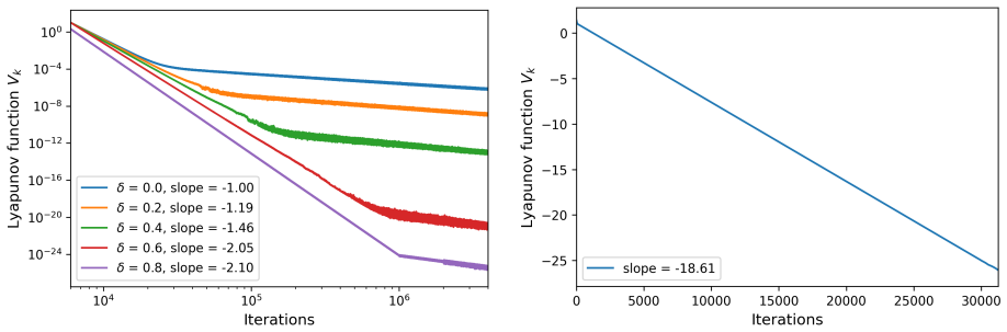
- The numerical experiments on SGD with Polyak-Ruppert averaging and stochastic bilevel optimization indicate the theoretical rates are actually observed in practice.
Reading between the lines
- A testable practical extension is to estimate the four exponents δij from data during running iterations and then set the step-size exponent a adaptively; the linear program gives a principled online schedule that should outperform any fixed schedule when noise decays non-uniformly across coordinates.
- The paper's general theorem hinges on a balancing condition that is only proven in the symmetric subcase; a natural check is whether that condition always holds, and if it fails for some asymmetric quadruple, the stated rate may require an extra constraint on the noise exponents.
- The exponential regime at δij=1 connects to overparametrized models where noise vanishes at the optimum; one could attempt to verify Theorem 2's constant-step-size prediction on real overparametrized least-squares or logistic regression problems as a direct validation.
- The time-dependent case suggests a broader conjecture: for general noise decaying as k^{-γ}, the optimal rate exponent may be the solution of a linear program analogous to m(x), with the exponential barrier appearing only when noise is a function of the state rather than the iteration count.
Editorial analysis
A structured set of objections, weighed in public.
Referee Report
Summary. The paper studies nonlinear two-time-scale stochastic approximation (1) under noise whose conditional variance decays either with the current residuals (Assumption 4, exponents δ_ij ∈ [0,1), with the boundary case δ_ij=1 in Assumption 5) or with the iteration counter (Assumption 6, exponents γ_i). Theorem 1 introduces a piecewise-linear function m(x), chooses step-size exponents a=argmax m and t=max m, and claims E[V_k] ≤ M/(k+k0)^t for all k, with t > 2/3 when δ_ij > 0. Corollary 1 works out the symmetric case and recovers the known 2/3 rate at δ=0. Theorem 2 claims an exponential rate under constant step sizes and large α/β when δ_ij=1. Theorem 3 gives a similar polynomial rate for time-dependent noise. The supplement supplies full proofs, including a telescoping-induction argument and a contraction argument.
Significance. If correct, the results provide an explicit, parameter-dependent convergence-rate formula for nonlinear two-time-scale SA and show that vanishing noise improves the classical O(k^{-2/3}) rate up to O(k^{-∞}) and exponential convergence in the δ=1 boundary case. The linear-programming construction of m(x) is elegant, and the proof details are largely supplied, with the symmetric case computed in closed form. The assumptions are clearly stated, and the predicted rates are falsifiable through the measured slopes in Section 5. I also verified that the balancing inequality (30)/(S27), which the text presents as an imposed condition, is in fact automatic: because t=m(a)=min_i L_i(a), each of the four inequalities is equivalent to t≤L_i(a). Thus the reader's weakest-assumption concern does not land.
major comments (2)
- [Theorem S2, Eqs. (S40)-(S43)] The expansion of the contraction coefficient in Theorem S2 does not match Lemma S3. Substituting α=ωβ into (S25) gives a β^2 coefficient of L_f^2ω^2 + 4L_λ^2L_g^2 + 2L_fL_λL_gω + (1/c)L_g^2(L_λ+2)ω + c4L_λ^2L_g^2(L_λ+1)^2/ω + L_g^2(2L_λ^2+L_λ+3), and a β^3 coefficient of (2/μ_g)L_f^2L_λ^2L_g^2(L_λ+1)^2ω^2 plus a noise term. The stated B1 and B2 lack the required powers of ω and 1/ω, so D2 and D3 are not the coefficients obtained from the proof, and the displayed e^{-ϵ} is not the actual contraction factor. The exponential-rate conclusion is still recoverable because D1(ω)→-μ_g/2 as ω→∞ and the higher-order terms vanish as β→0, but Eqs. (S40)-(S43) must be corrected.
- [Section 5, Figures 1-3 captions] The captions state 'All R-squares of the fitted slopes do not exceed 1e-6' (Figure 1), '0.01' (Figure 2), and '0.1' (Figure 3). If these are coefficients of determination, such values mean the straight-line fits explain almost none of the variance, which would contradict the text's claims that the measured slopes 'closely approximate' t and that the plots support the theory. Please replace these with the actual R^2 values (or another valid goodness-of-fit statistic) and describe the fitting procedure. This is essential for the experimental illustration to be meaningful.
minor comments (5)
- [Eq. (30)/(S27)] The four inequalities in (S27) are not derived. They are immediate from t=m(a)=min_i L_i(a): each inequality is algebraically equivalent to t≤L_i(a), where L_i are the four linear functions in (S26). Add this one-line verification in the supplement (and ideally a sentence in the main text) so readers do not mistake (S27) for an unproved balancing assumption.
- [Lemma 1 and Lemma 2] Both lemmas state 'for all k≥0' but condition on Q_{k-1}; Q_{-1} is not defined. Restrict to k≥1 or define Q_{-1}.
- [Abstract and Section 5] 'rate of polynomial delay' should probably be 'rate of polynomial decay'. Also, the experiment notation 'Γ'_kk ≡ Γ'' and 'γ_k ≡ γ' mixes subscripts; use one parameter name consistently.
- [Theorem 2 and Section 5] The contraction in Theorem 2 requires β to be sufficiently small for fixed ω (since 1+D1β+D2β^2+D3β^3<1 for small β). The surrounding text in Section 3 says 'β and α/β are sufficiently large' for Theorems 1 and 3; Theorem 2's regime should be stated explicitly as 'ω large, β small'.
- [Section 5] The sentence 'k0 increases rapidly with increasing (α,β) and affects the step sizes exponentially' is unclear; the step sizes are polynomial in k, and k0 is chosen via the bounds in (S32). Please rephrase to avoid confusion.
Circularity Check
No circularity: the balance condition (S27) is automatic from the definition of m(x); all convergence rates are derived analytically from the noise assumptions, with no fitted quantities fed back into the proof.
full rationale
The paper's derivation chain is self-contained. Theorem 1 (and its supplement Theorem S1) takes the noise exponents δ_ij as inputs and derives a Lyapunov bound E[V_k] ≤ M/(k+k0)^t by an induction whose constants are chosen to satisfy explicit inequalities; no experimental slope or fitted parameter enters the proof. The only potentially suspicious object is the linear program m(x) in Eq. (29)/(S26), described as 'set to satisfy' the balance condition (30)/(S27). This is not a fitted input or an imported self-citation: it is an internal analytic construction. Moreover, the balance condition is a direct consequence of the definition. Writing L1(x)=((1+δ11)x−δ11)/(1−δ11), L2(x)=x/(1−δ12), L3(x)=((2−δ21)(1−x))/(1−δ21), L4(x)=2(1−x)/(1−δ22), we have m(x)=min_i L_i(x). At x=a, t=m(a)=min_i L_i(a). Each of the four inequalities in (S27) is algebraically equivalent to t ≤ L_i(a); for example, −1+2a ≥ −1+a+t+(1−a−t)δ11 ⇔ t≤L1(a), and the other three reduce similarly. Since a is chosen as the argmax of m, all four hold identically. Thus the proof's use of (S27) is legitimate; the only lapse is that the supplement omits this one-line verification, which is a presentational omission, not circularity. Theorem 2's exponential rate is obtained by constructing a contraction factor e^{−ε}=1+D1(ω)β+D2(ω)β^2+D3(ω)β^3<1, with D1(ω)→−½μ_g as ω→∞; the existence of such β is a standard perturbation argument and does not fit data. The numerical section compares measured slopes to the theoretically predicted t rather than using those slopes to select constants in the theorems. No load-bearing self-citation occurs: prior work is cited for noise assumptions and baseline rates, but the main results are proved in the supplement from Assumptions 1–6. No circular step is present.
Assumptions & free parameters
assumptions (6)
- domain assumption Unique solution (x*,y*) and Lipschitz map lambda(y) exist (Assumption 1)
- domain assumption f is Lipschitz and strongly monotone in x; g is Lipschitz and 1-point strongly monotone (Assumptions 2-3)
- domain assumption State-dependent noise variance bounds scale as ||x_hat||^{2 delta} or ||y_hat||^{2 delta} with delta in [0,1) (Assumption 4)
- domain assumption Time-dependent noise variance bounds scale as k^{-gamma} (Assumption 6)
- ad hoc to paper Balance inequality (30)/(S27) holds for the linear-program maximizer a,t
- ad hoc to paper Noise time-exponents satisfy gamma1 - gamma2 in [-1, 1/2)
Cite this review
Pith. "Pith review of Convergence Rate in Nonlinear Two-Time-Scale Stochastic Approximation with State (Time)-Dependence." pith.science (2026). https://pith.science/paper/XYJ77XQ4
@misc{pith2026250911039,
  author       = {Pith},
  title        = {Pith review of: Convergence Rate in Nonlinear Two-Time-Scale Stochastic Approximation with State (Time)-Dependence},
  year         = {2026},
  howpublished = {\url{https://pith.science/paper/XYJ77XQ4}},
  note         = {Machine review of arXiv:2509.11039}
}
read the original abstract
The nonlinear two-time-scale stochastic approximation is widely studied under conditions of bounded variances in noise. Motivated by recent advances that allow for variability linked to the current state or time, we consider state- and time-dependent noises. We show that the Lyapunov function exhibits polynomial convergence rates in both cases, with the rate of polynomial delay depending on the parameters of state- or time-dependent noises. Notably, if the state noise parameters fully approach their limiting value, the Lyapunov function achieves an exponential convergence rate. We provide two numerical examples to illustrate our theoretical findings in the context of stochastic gradient descent with Polyak-Ruppert averaging and stochastic bilevel optimization.
Figures


Reference graph
Works this paper leans on
-
[1]
, " * write output.state after.block = add.period write newline
ENTRY address archivePrefix author booktitle chapter edition editor eid eprint howpublished institution isbn journal key month note number organization pages publisher school series title type volume year label extra.label sort.label short.list INTEGERS output.state before.all mid.sentence after.sentence after.block FUNCTION init.state.consts #0 'before.a...
-
[2]
write newline
" write newline "" before.all 'output.state := FUNCTION n.dashify 't := "" t empty not t #1 #1 substring "-" = t #1 #2 substring "--" = not "--" * t #2 global.max substring 't := t #1 #1 substring "-" = "-" * t #2 global.max substring 't := while if t #1 #1 substring * t #2 global.max substring 't := if while FUNCTION word.in bbl.in capitalize " " * FUNCT...
-
[3]
Abergel, F.; Anane, M.; Chakraborti, A.; Jedidi, A.; and Toke, I. M. 2016. Limit order books. Cambridge University Press
2016
-
[4]
Borkar, V. S. 1997. Stochastic approximation with two time scales. Systems & Control Letters, 29(5): 291--294
1997
-
[5]
Borkar, V. S. 2009. Stochastic approximation: a dynamical systems viewpoint, volume 48. Springer
2009
-
[6]
E.; and Nocedal, J
Bottou, L.; Curtis, F. E.; and Nocedal, J. 2018. Optimization methods for large-scale machine learning. SIAM review, 60(2): 223--311
2018
-
[7]
D.; Tong, X
Chen, X.; Lee, J. D.; Tong, X. T.; and Zhang, Y. 2020. Statistical inference for model parameters in stochastic gradient descent. Annals of Statistics, 48(1): 251--273
2020
-
[8]
Colson, B.; Marcotte, P.; and Savard, G. 2007. An overview of bilevel optimization. Annals of operations research, 153: 235--256
2007
Show all 34 references
-
[9]
Doan, T. T. 2022. Nonlinear two-time-scale stochastic approximation convergence and finite-time performance. IEEE Transactions on Automatic Control
2022
-
[10]
Doan, T. T. 2024. Fast Nonlinear Two-Time-Scale Stochastic Approximation: Achieving O (1/k) Finite-Sample Complexity. arXiv preprint arXiv:2401.12764
2024 arXiv
-
[11]
Ermoliev, Y. 1983. Stochastic quasigradient methods and their application to system optimization. Stochastics: An International Journal of Probability and Stochastic Processes, 9(1-2): 1--36
1983
-
[12]
Ermoliev, Y. 2009. Two-stage stochastic programming: quasigradient methodTwo-Stage Stochastic Programming: Quasigradient Method, 3955--3959. Boston, MA: Springer US. ISBN 978-0-387-74759-0
2009
-
[13]
Gatheral, J. 2011. The volatility surface: A Practitioner's Guide. John Wiley and Sons, Inc
2011
-
[14]
Han, Y.; Li, X.; and Zhang, Z. 2024. Finite-Time Decoupled Convergence in Nonlinear Two-Time-Scale Stochastic Approximation. arXiv preprint arXiv:2401.03893
2024 arXiv
-
[15]
Haykin, S. S. 2002. Adaptive filter theory. Pearson Education India
2002
-
[16]
Hu, J.; Doshi, V.; and Eun, D. Y. 2024. Central Limit Theorem for Two-Timescale Stochastic Approximation with Markovian Noise: Theory and Applications. arXiv preprint arXiv:2401.09339
2024 arXiv
-
[17]
Ilandarideva, S.; Juditsky, A.; Lan, G.; and Li, T. 2023. Accelerated stochastic approximation with state-dependent noise. arXiv preprint arXiv:2307.01497
2023 arXiv
-
[18]
Kaledin, M.; Moulines, E.; Naumov, A.; Tadic, V.; and Wai, H.-T. 2020. Finite time analysis of linear two-timescale stochastic approximation with Markovian noise. In Conference on Learning Theory, 2144--2203. PMLR
2020
-
[19]
L.; and Vidyasagar, M
Karandikar, R. L.; and Vidyasagar, M. 2023. Convergence Rates for Stochastic Approximation: Biased Noise with Unbounded Variance, and Applications. arXiv preprint arXiv:2312.02828
2023 arXiv
-
[20]
T.; Romberg, J.; and Maguluri, S
Khodadadian, S.; Doan, T. T.; Romberg, J.; and Maguluri, S. T. 2022. Finite sample analysis of two-time-scale natural actor-critic algorithm. IEEE Transactions on Automatic Control
2022
-
[21]
R.; and Tsitsiklis, J
Konda, V. R.; and Tsitsiklis, J. N. 2004. Convergence rate of linear two-time-scale stochastic approximation. The Annals of Applied Probability, 14(2): 796--819
2004
-
[22]
Lan, G. 2020. First-order and stochastic optimization methods for machine learning, volume 1. Springer
2020
-
[23]
Moulines, E.; and Bach, F. 2011. Non-asymptotic analysis of stochastic approximation algorithms for machine learning. Advances in neural information processing systems, 24
2011
-
[24]
Pham, K. 2010. New risk-averse control paradigm for stochastic two-time-scale systems and performance robustness. Journal of optimization theory and applications, 146: 511--537
2010
-
[25]
T.; and Juditsky, A
Polyak, B. T.; and Juditsky, A. B. 1992. Acceleration of stochastic approximation by averaging. SIAM journal on control and optimization, 30(4): 838--855
1992
-
[26]
Robbins, H.; and Monro, S. 1951. A stochastic approximation method. The annals of mathematical statistics, 400--407
1951
-
[27]
Ruppert, D. 1988. Efficient estimations from a slowly convergent Robbins-Monro process. Technical report, Cornell University Operations Research and Industrial Engineering
1988
-
[28]
M.; and Defazio, A
Sebbouh, O.; Gower, R. M.; and Defazio, A. 2021. Almost sure convergence rates for stochastic gradient descent and stochastic heavy ball. In Conference on Learning Theory, 3935--3971. PMLR
2021
-
[29]
Shen, H.; and Chen, T. 2022. A single-timescale analysis for stochastic approximation with multiple coupled sequences. Advances in Neural Information Processing Systems, 35: 17415--17429
2022
-
[30]
S.; Maei, H
Sutton, R. S.; Maei, H. R.; Precup, D.; Bhatnagar, S.; Silver, D.; Szepesv \'a ri, C.; and Wiewiora, E. 2009. Fast gradient-descent methods for temporal-difference learning with linear function approximation. In Proceedings of the 26th annual international conference on machin...
2009
-
[31]
S.; Szepesv \'a ri, C.; and Maei, H
Sutton, R. S.; Szepesv \'a ri, C.; and Maei, H. R. 2008. A convergent O(n) algorithm for off-policy temporal-difference learning with linear function approximation. Advances in neural information processing systems, 21(21): 1609--1616
2008
-
[32]
F.; Zhang, W.; Xu, P.; and Gu, Q
Wu, Y. F.; Zhang, W.; Xu, P.; and Gu, Q. 2020. A finite-time analysis of two time-scale actor-critic methods. Advances in Neural Information Processing Systems, 33: 17617--17628
2020
-
[33]
Xu, T.; Zou, S.; and Liang, Y. 2019. Two time-scale off-policy TD learning: Non-asymptotic analysis over Markovian samples. Advances in neural information processing systems, 32
2019
-
[34]
T.; and Romberg, J
Zeng, S.; Doan, T. T.; and Romberg, J. 2024. A two-time-scale stochastic optimization framework with applications in control and reinforcement learning. SIAM Journal on Optimization, 34(1): 946--976
2024
Reviewed August 4, 2026 · model on record in the stance chip above.
Discussion (0). Sign in to comment.